Dr. Vadym Zayets
v.zayets(at)gmail.com
My Research and Inventions
click here to see all content |

Dr. Vadym Zayetsv.zayets(at)gmail.com |
|
|
more Chapters on this topic:IntroductionTransport Eqs.Spin Proximity/ Spin InjectionSpin DetectionBoltzmann Eqs.Band currentScattering currentMean-free pathCurrent near InterfaceOrdinary Hall effectAnomalous Hall effect, AMR effectSpin-Orbit interactionSpin Hall effectNon-local Spin DetectionLandau -Lifshitz equationExchange interactionsp-d exchange interactionCoercive fieldPerpendicular magnetic anisotropy (PMA)Voltage- controlled magnetism (VCMA effect)All-metal transistorSpin-orbit torque (SO torque)What is a hole?spin polarizationCharge accumulationMgO-based MTJMagneto-opticsSpin vs Orbital momentWhat is the Spin?model comparisonQuestions & AnswersEB nanotechnologyReticle 11
more Chapters on this topic:IntroductionTransport Eqs.Spin Proximity/ Spin InjectionSpin DetectionBoltzmann Eqs.Band currentScattering currentMean-free pathCurrent near InterfaceOrdinary Hall effectAnomalous Hall effect, AMR effectSpin-Orbit interactionSpin Hall effectNon-local Spin DetectionLandau -Lifshitz equationExchange interactionsp-d exchange interactionCoercive fieldPerpendicular magnetic anisotropy (PMA)Voltage- controlled magnetism (VCMA effect)All-metal transistorSpin-orbit torque (SO torque)What is a hole?spin polarizationCharge accumulationMgO-based MTJMagneto-opticsSpin vs Orbital momentWhat is the Spin?model comparisonQuestions & AnswersEB nanotechnologyReticle 11
more Chapters on this topic:IntroductionTransport Eqs.Spin Proximity/ Spin InjectionSpin DetectionBoltzmann Eqs.Band currentScattering currentMean-free pathCurrent near InterfaceOrdinary Hall effectAnomalous Hall effect, AMR effectSpin-Orbit interactionSpin Hall effectNon-local Spin DetectionLandau -Lifshitz equationExchange interactionsp-d exchange interactionCoercive fieldPerpendicular magnetic anisotropy (PMA)Voltage- controlled magnetism (VCMA effect)All-metal transistorSpin-orbit torque (SO torque)What is a hole?spin polarizationCharge accumulationMgO-based MTJMagneto-opticsSpin vs Orbital momentWhat is the Spin?model comparisonQuestions & AnswersEB nanotechnologyReticle 11
more Chapters on this topic:IntroductionTransport Eqs.Spin Proximity/ Spin InjectionSpin DetectionBoltzmann Eqs.Band currentScattering currentMean-free pathCurrent near InterfaceOrdinary Hall effectAnomalous Hall effect, AMR effectSpin-Orbit interactionSpin Hall effectNon-local Spin DetectionLandau -Lifshitz equationExchange interactionsp-d exchange interactionCoercive fieldPerpendicular magnetic anisotropy (PMA)Voltage- controlled magnetism (VCMA effect)All-metal transistorSpin-orbit torque (SO torque)What is a hole?spin polarizationCharge accumulationMgO-based MTJMagneto-opticsSpin vs Orbital momentWhat is the Spin?model comparisonQuestions & AnswersEB nanotechnologyReticle 11
more Chapters on this topic:IntroductionScatteringsSpin-polarized/ unpolarized electronsSpin statisticselectron gas in Magnetic FieldFerromagnetic metalsSpin TorqueSpin-Torque CurrentSpin-Transfer TorqueQuantum Nature of SpinQuestions & Answers
more Chapters on this topic:IntroductionTransport Eqs.Spin Proximity/ Spin InjectionSpin DetectionBoltzmann Eqs.Band currentScattering currentMean-free pathCurrent near InterfaceOrdinary Hall effectAnomalous Hall effect, AMR effectSpin-Orbit interactionSpin Hall effectNon-local Spin DetectionLandau -Lifshitz equationExchange interactionsp-d exchange interactionCoercive fieldPerpendicular magnetic anisotropy (PMA)Voltage- controlled magnetism (VCMA effect)All-metal transistorSpin-orbit torque (SO torque)What is a hole?spin polarizationCharge accumulationMgO-based MTJMagneto-opticsSpin vs Orbital momentWhat is the Spin?model comparisonQuestions & AnswersEB nanotechnologyReticle 11
more Chapters on this topic:IntroductionTransport Eqs.Spin Proximity/ Spin InjectionSpin DetectionBoltzmann Eqs.Band currentScattering currentMean-free pathCurrent near InterfaceOrdinary Hall effectAnomalous Hall effect, AMR effectSpin-Orbit interactionSpin Hall effectNon-local Spin DetectionLandau -Lifshitz equationExchange interactionsp-d exchange interactionCoercive fieldPerpendicular magnetic anisotropy (PMA)Voltage- controlled magnetism (VCMA effect)All-metal transistorSpin-orbit torque (SO torque)What is a hole?spin polarizationCharge accumulationMgO-based MTJMagneto-opticsSpin vs Orbital momentWhat is the Spin?model comparisonQuestions & AnswersEB nanotechnologyReticle 11
more Chapters on this topic:IntroductionTransport Eqs.Spin Proximity/ Spin InjectionSpin DetectionBoltzmann Eqs.Band currentScattering currentMean-free pathCurrent near InterfaceOrdinary Hall effectAnomalous Hall effect, AMR effectSpin-Orbit interactionSpin Hall effectNon-local Spin DetectionLandau -Lifshitz equationExchange interactionsp-d exchange interactionCoercive fieldPerpendicular magnetic anisotropy (PMA)Voltage- controlled magnetism (VCMA effect)All-metal transistorSpin-orbit torque (SO torque)What is a hole?spin polarizationCharge accumulationMgO-based MTJMagneto-opticsSpin vs Orbital momentWhat is the Spin?model comparisonQuestions & AnswersEB nanotechnologyReticle 11
more Chapters on this topic:IntroductionTransport Eqs.Spin Proximity/ Spin InjectionSpin DetectionBoltzmann Eqs.Band currentScattering currentMean-free pathCurrent near InterfaceOrdinary Hall effectAnomalous Hall effect, AMR effectSpin-Orbit interactionSpin Hall effectNon-local Spin DetectionLandau -Lifshitz equationExchange interactionsp-d exchange interactionCoercive fieldPerpendicular magnetic anisotropy (PMA)Voltage- controlled magnetism (VCMA effect)All-metal transistorSpin-orbit torque (SO torque)What is a hole?spin polarizationCharge accumulationMgO-based MTJMagneto-opticsSpin vs Orbital momentWhat is the Spin?model comparisonQuestions & AnswersEB nanotechnologyReticle 11
|
Measurement of strength of Spin-Orbit Interaction
Spin and Charge TransportSpin-orbit interaction refers to a magnetic field of relativistic origin experienced by an electron while moving within an electric field.The spin-orbit interaction stands as one of the most crucial fundamental effects in physics, holding a pivotal role in numerous phenomena within Solid State Physics.
|
(video): |
|||||||||||||||||||||||||||||||||||
|---|---|---|---|---|---|---|---|---|---|---|---|---|---|---|---|---|---|---|---|---|---|---|---|---|---|---|---|---|---|---|---|---|---|---|---|
|
|||||||||||||||||||||||||||||||||||
| click on image to play it |
Coefficient of spin-orbit interaction kSO is a measure of strength of the spin- orbit interaction |
|---|
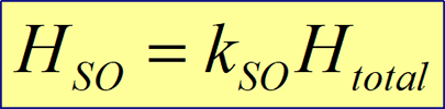 |
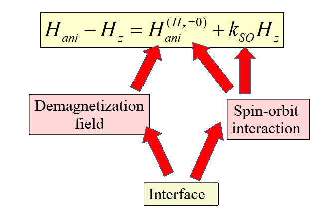
Only parameter, which describes the strength of spin- orbit interaction, is the magnetic field Hso of spin- orbit interaction. The strength of Hso is proportional to the total applied magnetic field Htotal. The proportionality coefficient is called the coefficient of spin- orbit interaction and which gives the strength of the spin- orbit interaction. |
| The total applied magnetic field is the sum of intrinsic and external magnetic field. |
![]() The coefficient of spin-orbit interaction kSO, which gives the strength of the spin- orbit interaction. kSO is the proportionality coefficient between the magnetic field Hso of spin- orbit interaction and the total applied magnetic field Htotal (internal plus external magnetic fields).
The coefficient of spin-orbit interaction kSO, which gives the strength of the spin- orbit interaction. kSO is the proportionality coefficient between the magnetic field Hso of spin- orbit interaction and the total applied magnetic field Htotal (internal plus external magnetic fields).
Measurement of strength of spin-orbit interaction |
|---|
 |
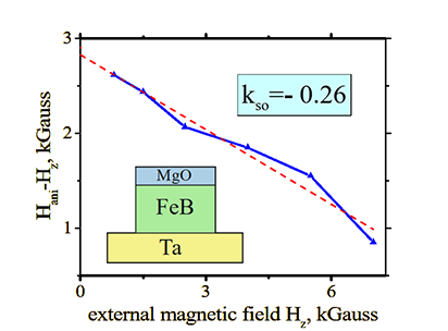
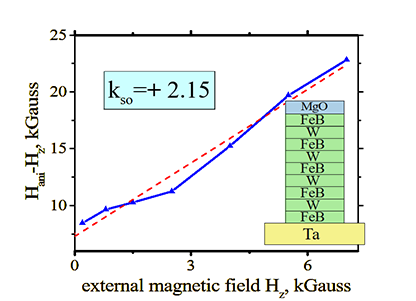
Eq. 45. Anisotropy field Hani is linearly increases when an external magnetic field Hz is applied along the magnetic easy axis. The proportionality coefficient between Hani and Hz is the coefficient of the spin orbit interaction kSO. |
| (measurement method) The anisotropy field Hani is measured as a function of an external magnetic field Hz applied along the magnetic easy axis. The proportionality coefficient gives kSO |
| (math) The detailed math of how to obtain this equation is here |
![]() The measurement of the strength of the spin- orbit interaction is relatively simple and straightforward.
The measurement of the strength of the spin- orbit interaction is relatively simple and straightforward.
The magnetic field of spin-orbit interaction Hso holds the magnetization along the magnetic easy axis. A measurement of how strongly the magnetization is held along its easy axis evaluates the strength of the spin- orbit interaction.
For this purpose, an external magnetic field is applied along the hard axis and, therefore, perpendicular to the easy axis forcing the magnetization to tilt out from the easy axis. The stronger the spin- orbit interaction is, the harder it is to tilt the magnetization.
The anisotropy field is a magnetic field, at which the magnetization is fully tilted along the hard axis, and is a good measure of the spin-orbit interaction.
If additionally an external magnetic field is applied along the easy axis, the spin- orbit interaction becomes stronger and, correspondingly, the anisotropy field becomes larger. As you can see, the anisotropy field is linearly proportional to the strength of the spin-orbit interaction. Therefore, a measurement of anisotropy field versus the external field,gives the strength of the spin- orbit interaction.
Measurement of strength of spin-orbit interaction |
|---|
 |
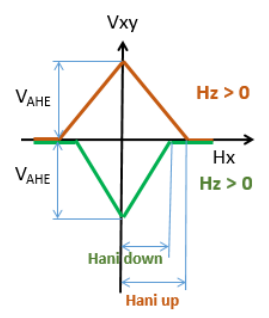
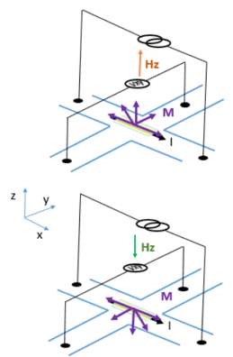
Two magnetic fields are independently controlled in this measurement. The in-plane magnetic field Hx is applied in-plane and, therefore, perpendicularly to the easy axis. Hz is applied along the easy axis. |
| (measurement method) For each fixed Hz, Hx is scanned and the magnetization tilting angle is measured. From this dependence, the value of Hani is evaluated for each Hz. From linear dependence Hani vs. Hz, kSO is evaluated |
 (key feature of the measurement): Two magnetic fields (along Hz and perpendicular Hx to the easy axis) are applied and independently controlled
(measurement method)
![]() (step 1): For each fixed Hz, Hx is scanned and the magnetization tilting angle is measured.
(step 1): For each fixed Hz, Hx is scanned and the magnetization tilting angle is measured.
![]() (step 2): From the dependence of Hani vs. Hx, the value of Hani is evaluated for each Hz.
(step 2): From the dependence of Hani vs. Hx, the value of Hani is evaluated for each Hz.
![]() (step 3):From linear dependence Hani vs. Hz, kSO is evaluated
(step 3):From linear dependence Hani vs. Hz, kSO is evaluated
Relation between spin-orbit interaction and anisotropy field |
|---|
 |
When some conditions at a nanomagnet interface are changing, it affects both the strength of spin orbit interaction kSO and demagnetization field Hdemag. Since the anisotropy field Hani depends on both kSO and Hdemag, the anisotropy field changes as well. However, the polarity change of Hani may be different according to whether the kSO or Hdemag contribution to anisotropy field is dominated for the specific nanomagnet. |
| When polarity of change of Hani is the same as that of kSO, the spin- orbit contribution dominates. |
| When polarity of change of Hani is opposite to that of kSO, the demagnetization contribution dominates. |
| click on image to enlarge it |
There are two parameters, which are evaluated from the measured linear dependence of Fig.41: (parameter 1): coefficient kSO of spin orbit interaction (the slope of the line) and (parameter 2): anisotropy field in absence of external field or simply the anisotropy field Hani ( the offset of the line)
Both kSO and Hani depend on a variety of nanomagnet parameters such as interface roughness, nanomagnet thickness, current, gate voltage etc.
It is important, the dependencies of kSO and Hani are not independent.
![]() (reason):
(reason):
The anisotropy field is proportional to the strength of the spin- orbit interaction and the internal magnetic field Hint:
![]()
The internal magnetic field is the field along the magnetization M minus the demagnetization field Hdemag and plus the magnetic field of spin- orbit interaction HSO:
![]()
Therefore, the anisotropy field is proportional to the coefficient of spin-orbit interaction and the demagnetization field:
![]()
(note) Usually kSO and Hdemag increase or decrease simultaneously. As a consequence, the anisotropy field Hani can either increase or decrease depending which contribution kSO or Hdemag to Hani is larger
![]() Factors, which affect kSO and Hdemag:
Factors, which affect kSO and Hdemag:
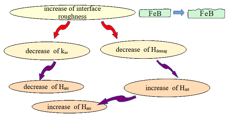
![]() (factor 1): interface roughness (see below)
(factor 1): interface roughness (see below)
(rougher interface) → (kSO is smaller) & (Hdemag is smaller) ⇒ (Hani is either smaller or larger)
The dependence of on the interface roughness is different for a nanomagnet containing one or several ferromagnetic layers.
a single-layer nanomagnet: (rougher interface) →(Hani is smaller)
a multi-layer nanomagnet: (rougher interface) →(Hani is larger)
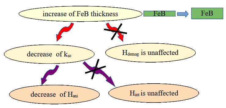
![]() (factor 2): nanomagnet thickness (see below)
(factor 2): nanomagnet thickness (see below)
(thicker nanomagnet) → (kSO is smaller) & (Hdemag is the same) ⇒ (Hani is smaller )
![]() (factor 3): polarity of applied magnetic field (see below)
(factor 3): polarity of applied magnetic field (see below)
(larger change with reversal of H) → ( ΔkSO is larger) & (ΔHdemag is the same) ⇒ (ΔHani is larger )
![]() (factor 4): Electrical current. SOT effect (see below)
(factor 4): Electrical current. SOT effect (see below)
(a larger current) → (kSO is ) & (Hdemag is ) ⇒ (Hani is )
![]() (factor 5): Gate voltage. VCMA effect (see below)
(factor 5): Gate voltage. VCMA effect (see below)
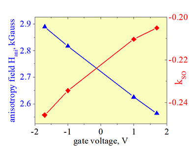
(a larger positive gate voltage) → (kSO is larger) & (Hdemag is smaller) ⇒ (Hani is smaller)
Measurement of internal magnetic field |
|---|
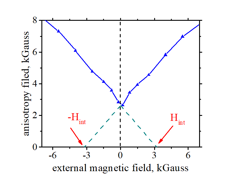 |
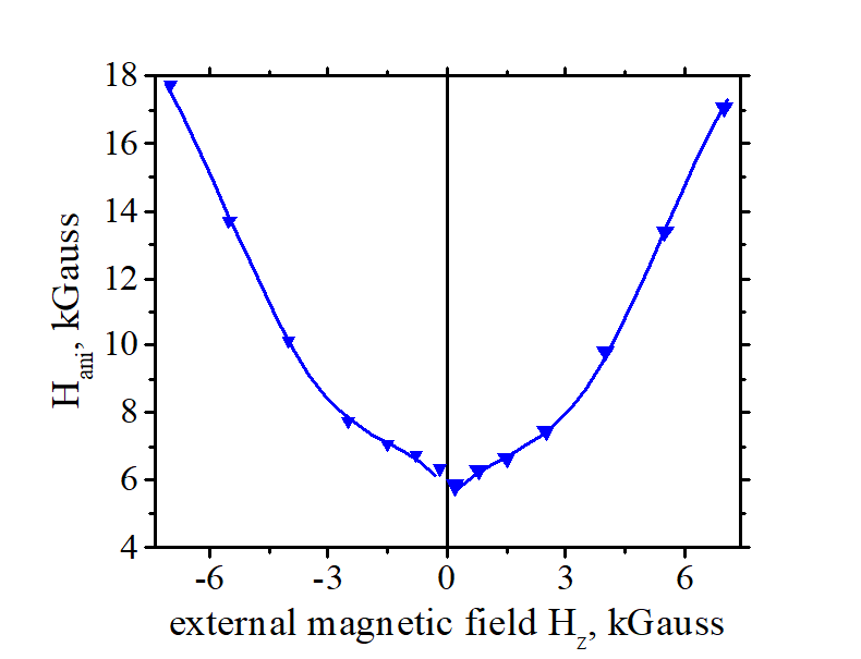
Extending measured linear dependence of anisotropy Hani vs. external magnetic field Hz till value Hani=0, gives the value of the internal magnetic field Hint |
| The case Hani=0 corresponds to the case when there is no magnetic anisotropy and, therefore, when the anisotropy field equals zero and when there is no internal field. |
| click on image to enlarge it |
The magnetic field, which holds the magnetization along its easy axis, is called the internal magnetic field.
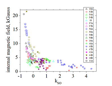
![]() (fact) The measured internal magnetic field in a FeCoB nanomagnet is in range between 2.5-5 kG. However it can be as large as 15 kG in a single- layer FeCoB nanomagnet and can be less than 1 kG in a multilayer nanomagnet.
(fact) The measured internal magnetic field in a FeCoB nanomagnet is in range between 2.5-5 kG. However it can be as large as 15 kG in a single- layer FeCoB nanomagnet and can be less than 1 kG in a multilayer nanomagnet.
![]() (how to measure the internal magnetic field)
(how to measure the internal magnetic field)
The anisotropy filed depends linearly on the external magnetic field Hz, which is applied along easy axis
![]()
In absence of external magnetic field Hz, only the internal magnetic field Hint holds the magnetization along the magnetic easy axis and the anisotropy field is linearly proportional to the internal magnetic field Hint. Since both the external and internal magnetic field are just the magnetic field and, therefore, should have the similar force on the spin, Eq. (41.1) can be written as
![]()
Similar to the external magnetic field Hz, the internal magnetic field Hint also has the bulk contribution, which should be considered. Then, correct form of Eq. (41.2) would be
![]()
Comparison of Eqs (41.1) and (41.2) gives the internal magnetic field Hint as
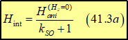
In the case when there is no external magnetic field Hz =0 and no internal magnetic field Hint=0, the anisotropy field eqauls zero (See Eq. 41.2a) and there is no magnetic anisotropy
![]() (fact) In vacuum, there is no magnetic anisotropy. Therefore, the anisotropy field equals zero and there is no internal field.
(fact) In vacuum, there is no magnetic anisotropy. Therefore, the anisotropy field equals zero and there is no internal field.
| Measured internal magnetic field in FeCoB nanomagnets | Samples. Thickness in nm shown in blankets |
|---|---|
 |
 |
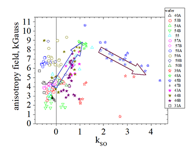
| Fig 44 The internal magnetic field vs. coefficient kSO of spin- orbit interaction systematically measured in FeCoB nanomagnets of different thickness, size, structure, composition. | Dots of the same color and shape correspond to nanomagnet fabricated at different places of the same wafer. Stars show multilayer nanomagnets, which contain several ferromagnetic layers. |
| The internal magnetic field is stronger for single- layer nanomagnets and weaker for multi-layer nanomagnets (shown by stars). | The nanomagnet of a different width and length in range from 50 x 50 nm to 3000 nm x 3000 nm are shown. |
(contribution 1) : Magnetic field along magnetization M
(contribution 2) : Demagnetization field
(contribution 3) : Magnetic field HSO of the spin-orbit interaction
![]() (fact) The electrons in the bulk of a nanomagnet and at the interface experience a very different internal magnetic field Hint, because they experience a very different magnetic field HSO of the spin-orbit interaction
(fact) The electrons in the bulk of a nanomagnet and at the interface experience a very different internal magnetic field Hint, because they experience a very different magnetic field HSO of the spin-orbit interaction
(factor 1) : Magnetization M
A nanomagnet, which has a larger magnetization, often has a larger Hint, because of larger contribution 1. However, other factors can reverse this tendency.
(factor 2) : Magnetic anisotropy. Anisotropy field Hani
A harder nanomagnet has a larger Hint. The anisotropy field Hani is linearly proportional to the internal magnetic field Hint
(factor 3) : Roughness and sharpness of an interface
Both the demagnetization field and the magnetic field of Spin-orbit interaction substantially depend on the perfection of the interface.
(factor 4) : Thickness of a nanomagnet
The strength of spin- orbit interaction is substantially different for the electrons in the bulk of a nanomagnet and at the interface. The bulk contribution is stronger for a thicker nanomagnet and the interface contribution is stronger for a thinner nanomagnet
(factor 5) : Structure of a nanomagnet
The demagnetization field is substantially in a multilayer nanomagnet than in a single layer nanomagnet. As a consequence, the internal magnetic field in a multilayer nanomagnet is smaller than in a single layer nanomagnet. This is because the effect of interfacial imperfections, which reduces the demagnetization field, is less prominent in a multilayer nanomagnet.
![]() Why is the internal magnetic field in a multilayer nanomagnet substantially smaller than in a multi- layer nanomagnet?
Why is the internal magnetic field in a multilayer nanomagnet substantially smaller than in a multi- layer nanomagnet?
It is because of a larger demagnetization field. The larger the number of interfaces is, the more efficiently the demagnetization field is created. In an ideal non- existed case of 100% efficiency of creation of the demagnetization (e.g. ideally- smooth ideally- planar ideally- sharp interface), the demagnetization field exactly equals the magnetization field and, as a consequence, the internal magnetic field becomes zero.
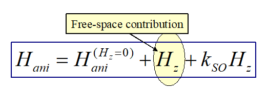
free-space contribution to Hani |
|---|
 |
|
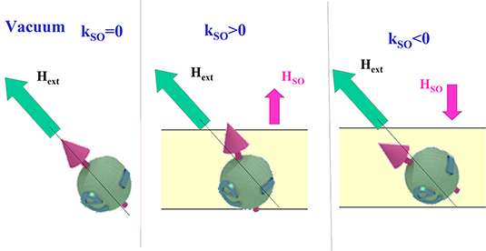 |
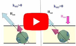
| (left) In vacuum, the spin is always aligned precisely along the external magnetic field. In a nanomagnet, the magnetic field HSO of spin- orbit interaction tilts the spin out of the direction of the external magnetic field Hext |
| (center) When the coefficient kSO of spin-orbit interaction is positive, the spin is tilted towards the surface normal. (right) When the coefficient kSO of spin-orbit interaction is positive, the spin is tilted towards the in-plane direction. |
| click on image to enlarge it |
The origin of the free-space contribution to Hani is the simple and obvious fact that in vacuum the spins always align perfectly along the magnetic field.
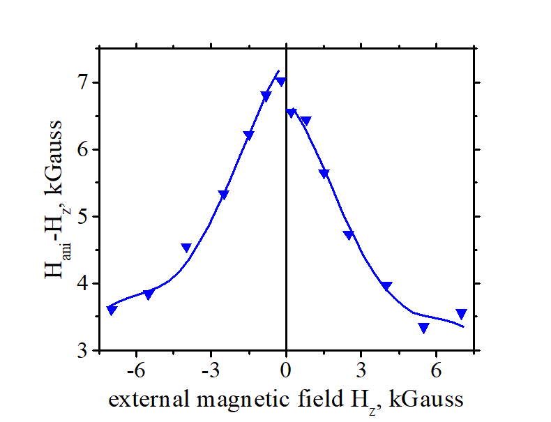
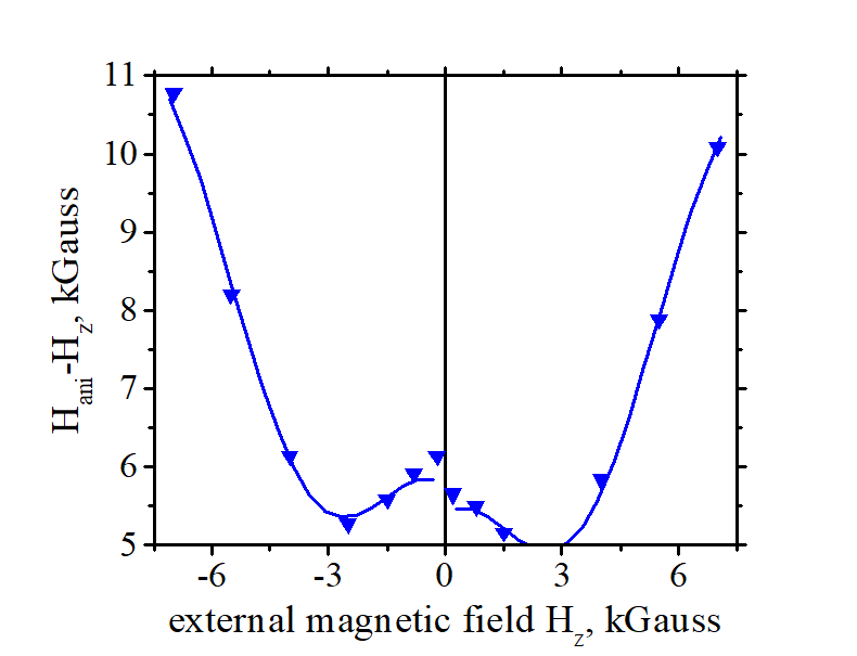
![]() (fact): Because of the free-space contribution, the dependence of Hani -Hz vs. Hz is more informative than the dependence of Hani vs. Hz
(fact): Because of the free-space contribution, the dependence of Hani -Hz vs. Hz is more informative than the dependence of Hani vs. Hz
In vacuum, the spin is always aligned exactly along the external magnetic field.
In a nanomagnet, the external field also creates the SO magnetic field.
When this field is directed along an external field, kSO is positive.
When SO field is directed opposite to external field, kSO is negative
Excluding free-space contribution |
|||||||||
|---|---|---|---|---|---|---|---|---|---|
with free- space contribution |
|||||||||
|
|||||||||
| The presence of non-informative free-space contribution masks crucial properties embedded within this measured dependence. These properties include the slope of the line, which directly relates to the strength of the spin-orbit interaction, as well as the oscillations and disparities observed during magnetization reversal. | |||||||||
without free space contribution |
|||||||||
|
|||||||||
| Upon eliminating the non-informative free-space contribution, the polarity and strength of the spin-orbit interaction (reflected by line slopes), the amplitude and period of oscillation, and the distinctions arising from magnetization reversal become distinctly visible and unequivocally clear. | |||||||||
| click on image to enlarge it |
The strength of the spin-orbit interaction exhibits oscillations as the external magnetic field increases. The oscillation is due to a periodic dependence of spin- orbit interaction on the magnetic field.
The oscillations of the strength of spin- orbit interaction are very clear in experimental measurements and are observed for any nanomagnet, which I have measured.
| Oscillations of the strength of spin- orbit interaction | |||||||||
|---|---|---|---|---|---|---|---|---|---|
|
|||||||||
| (oscillations): There are clear oscillations on top of the linear dependence. The oscillation is due to a periodic dependence of spin- orbit interaction on the magnetic field. The oscillation is a feature of an interface and is stronger when interface contribution is larger and the bulk contribution is weaker | |||||||||
| click on image to enlarge it |
 (How to measure?)
Measured dependence of anisotropy field Hani vs. external magnetic field Hz has two components: (component 1): linear increase; (component 2) oscillating component
| Origin of Oscillations of the strength of spin- orbit interaction under an external magnetic field |
|---|
| The oscillations are very clear in experimental measurements and are observed for any nanomagnet, which I have measured. |
| (close guess): The strength of spin- orbit interactions increases because orbital deformation under the Lorentz force in the magnetic field is different for parts of orbitals corresponding to the electron rotation in the clockwise and counterclockwise directions. The deformations are influenced by the other orbitals. The influence by each orbitals might be optimum at some value of the magnetic field making the maximum of the strength of the spin- orbit interaction. Each orbital has a different maximum. As a result, the dependence looks periodical. |
| As 2023.06, there are no enough experimental measurements to clarify the Origin of observed Oscillations |
Two components of dependence Hani vs. Hz
![]() (component 1 of Hani vs Hz) (general (main) dependency): linear dependency
(component 1 of Hani vs Hz) (general (main) dependency): linear dependency
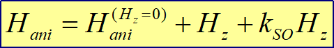
The strength of spin-orbit interaction is linearly proportional to the external magnetic field Hz. As a result, the anisotropy field Hani can be expressed as
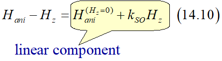
where Hz are external magnetic field, Hani (Hz =0) is the anisotropy field in absence of the external magnetic field and kSO is the coefficient of spin- orbit interaction.
![]() (component 2 of Hani vs Hz) (minor dependency): oscillating dependency
(component 2 of Hani vs Hz) (minor dependency): oscillating dependency
The strength of the spin-orbit interaction exhibits oscillations as the external magnetic field increases. These oscillations serve as a minor contribution to the primary linear dependence of Hani vs. Hz, which slope is determined by the strength of the spin-orbit interactions.

where Aosc is amplitude of oscillation, Hperiod is the period of oscillations (the magnetic field, after which the oscillations repeats itself), Hphase is the phase of oscillations, Hdecay is field for the decay of oscillations.

![]() (fact) This formula give a a perfect fitting of measured data for all nanomagnets I have measured so far.
(fact) This formula give a a perfect fitting of measured data for all nanomagnets I have measured so far.
The observed oscillations correspond to variations in the strength of the spin-orbit interaction as the external magnetic field increases.
There are clear oscillations on top of the linear dependence. The oscillation is due to a periodic dependence of spin- orbit interaction on the magnetic field. The oscillation is a feature of an interface and is stronger when interface contribution is larger and the bulk contribution is weaker
 (interfacial origin of oscillations): The oscillations are weaker for a thicker nanomagnet, where the bulk contribution dominates, and stronger for a thinner nanomagnet, in which the interfacial contribution dominates. It clearly indicates the interfacial origin of the oscillations.
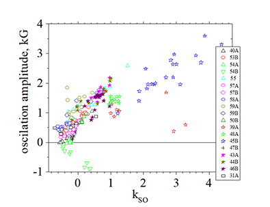
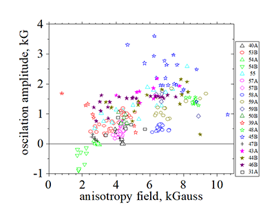
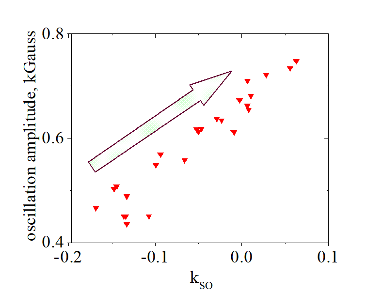
 (linear proportionality of oscillation amplitude to the strength of spin- orbit interaction): The measured amplitude Aosc of oscillation is linear proportional to the strength of the spin-orbit interaction or , the same, to the coefficient of SO (kso). It is true for nanomagnets fabricated on a single wafer (See Fig.19) and for the nanomagnets of a different size, material, composition, thickness, structure fabricated on different wafer (See Figs. 22b,22c below). The slope of dependence Aosc vs. kSO is positive. Since the positive contribution to kSO is from the interface, the positive means again the interfacial origin of the oscillations.
| Distribution of oscillation amplitude vs. strength of spin orbit interaction | Raw data |
|---|---|
 |
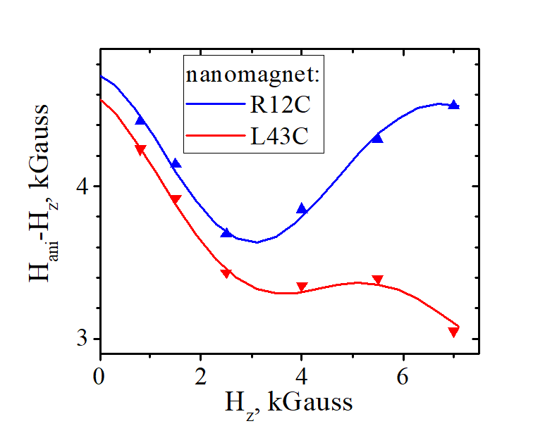 |
| Fig. 19 Measured amplitude of oscillation of the strength of spin- orbit interaction vs. measured coefficient kso of spin-orbit interaction. Each dot corresponds to a measurement of one individual nanomagnet fabricated at a different place of one wafer. The variations of amplitude and kso are due to variations of roughness and thickness over the wafer. Arrow shows the tendency. | Fig.19a. Measured anisotropy field Hani vs. external magnetic field Hz for two nanomagnets (R12C & L43C) fabricated on the same wafer Volt57B. Dots are measured data, lines are fitting. The fitting is perfect in both cases. Nanomagnet R12C has a stronger spin-orbit (kso= + 0.06) and a larger oscillation amplitude of 0.75 kG. Nanomagnet L43C has a weaker spin-orbit (kso= - 0.17)(slope is negative) and a smaller oscillation amplitude of 0.46 kG. |
The dependence is clearly linear and the slope is positive!! |
There is a clear correspondence between slope and oscillation amplitude!!! |
| wafer Volt57B :Ta(5 nm)/ FeCoB( x=0.5 1.1 nm) (click here fore more details) | click on image to enlarge it |
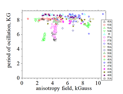
![]() (period of oscillation): The period Hperiod of oscillation is nearly identical for all nanomagnets and equals approximately 8 kGauss (See Fig. 21c below).
(period of oscillation): The period Hperiod of oscillation is nearly identical for all nanomagnets and equals approximately 8 kGauss (See Fig. 21c below).
![]() (phase of oscillations): The non-zero measured phase Hphase of oscillation means that the 1st maximum of oscillation is not at Hz=0, but is slightly shifted. For all measured nanomagnets, the phase Hphase is in range 0.1-0.2 kGauss.
(phase of oscillations): The non-zero measured phase Hphase of oscillation means that the 1st maximum of oscillation is not at Hz=0, but is slightly shifted. For all measured nanomagnets, the phase Hphase is in range 0.1-0.2 kGauss.
![]() (decay of oscillations): The amplitude of oscillation decreases when the external magnetic field increases. Typically, at a half period of oscillation the oscillation amplitude decreases for about 40%. Some nanomagnets do not show any decrease of the oscillation amplitude and some nanomagnets show even an increase of the oscillation amplitude. The decrease or increase of the oscillation amplitude substantially depends on size, material, composition, thickness, and structure of the nanomagnet.
(decay of oscillations): The amplitude of oscillation decreases when the external magnetic field increases. Typically, at a half period of oscillation the oscillation amplitude decreases for about 40%. Some nanomagnets do not show any decrease of the oscillation amplitude and some nanomagnets show even an increase of the oscillation amplitude. The decrease or increase of the oscillation amplitude substantially depends on size, material, composition, thickness, and structure of the nanomagnet.
 The data of measured Hani, kSO , Hperiod, , Hphase, Hdecay for all nanomagnets, which I have measured so far, can be found in this origin file: AllSampleHani.opj
 (systematic error due to oscillations): The amplitude of oscillation in a nanomagnet with a strong spin- orbit interaction (kso>0.2) becomes very large of about 1 kGauss and larger. It creates ambiguity of the fitting of the experimental data. The oscillating contribution may become dominating and there may be an ambiguity to distinguish the linear contribution. This can create some systematic error in measurement of kSO and Hani. See, for example, Fig. 19a above.
 (fact) The oscillations of the strength of the spin- orbit interaction are large!!!
 Especially, the oscillations are large in nanomagnets with a strong interfacial anisotropy and with a large spin-orbit interaction
| Systematic measurements in FeCoB nanomagnets | |||||||||||||||||||||
|---|---|---|---|---|---|---|---|---|---|---|---|---|---|---|---|---|---|---|---|---|---|
Comparison of data of many different nanomagnets of a different size, material, composition, thickness, structure. |
|||||||||||||||||||||
|
|||||||||||||||||||||
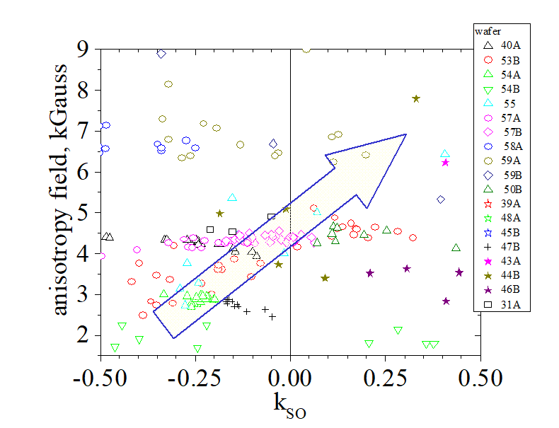
| Dots of the same color and shape correspond to nanomagnet fabricated at different places of the same wafer. Stars show multilayer nanomagnets, which contain several ferromagnetic layers. | |||||||||||||||||||||
| click on image to enlarge it |
There are small variations of thickness and interface roughness from a point to a point at the same wafer. Parameters of nanomagnets, which are fabricated at different places( e.g. at center or at edge of wafer or just at two close neighbor points), vary due to a variation of the interface roughness and due to a variation of the nanomagnet thickness.
![]() The strength of spin orbit interaction and the demagnetization field are two parameters, which are directly affected by variations of thickness and roughness. Because of the variations of these two parameters, the anisotropy field Hani and the intrinsic magnetic field are affected by variations of thickness and roughness as well.
The strength of spin orbit interaction and the demagnetization field are two parameters, which are directly affected by variations of thickness and roughness. Because of the variations of these two parameters, the anisotropy field Hani and the intrinsic magnetic field are affected by variations of thickness and roughness as well.
 (effect of interface roughness):
(kSO & Hdemag): A rougher interface reduces both the strength of the spin- orbit interaction kSO and the demagnetization field Hdemag.
(anisotropy field Hani): A rougher interface may either decrease or increase the anisotropy field.
When the contribution of kSO to Hani dominates, a rougher interface causes a decrease of Hani. Hani is flowing the change of kSO. E.g. it is a case of a single- layer nanomagnet.
When the contribution of Hdemag to Hani dominates, a rougher interface causes an increase of Hani. Hani is flowing the change of Hdemag. E.g. it is a case of a multi- layer nanomagnet.
(intrinsic magnetic field Hint): Hint is affected strongly by the roughness. The internal magnetic field Hint is just a difference between the magnetic field along magnetization and the demagnetization field. For an ideally- flat surface (a non-existed subject), the demagnetization field exactly equal to the magnetization and, therefore, the becomes zero. A rougher interface reduces the demagnetization field and, therefore, increases the internal magnetic filed.
(SO strength kSO): There are different contributions to the total strength of SO from the bulk and the interface. As a nanomagnet become thinner .
(anisotropy field Hani): A rougher interface may either decrease or increase the anisotropy field.
(intrinsic magnetic field Hint): Hint is not affected strongly by the nanomagnet thickness when the interface roughness and other parameters remains the same.
![]() (Why there is a thickness variation): In MRAM applications, the FeCoB nanomagnet typically has a thickness of 1 nm. Considering that the interatomic distance in FeCoB is approximately 0.1 nm, this implies that there are merely around 10-15 atomic layers spanning the thickness. Consequently, the absence of even a single atom can lead to a significant variation of 5-10% in the thickness of the nanomagnet.
(Why there is a thickness variation): In MRAM applications, the FeCoB nanomagnet typically has a thickness of 1 nm. Considering that the interatomic distance in FeCoB is approximately 0.1 nm, this implies that there are merely around 10-15 atomic layers spanning the thickness. Consequently, the absence of even a single atom can lead to a significant variation of 5-10% in the thickness of the nanomagnet.
Distribution of strength of spin- orbit interaction kSO and anisotropy field Hani due to variations of thickness and roughness is not random, but linear. |
|---|
 |
fact for nanomagnets fabricated at different places of one wafer |
| click on image to enlarge it |
Two independent parameters, which are affect by variations of the nanomagnet thickness and the interface roughness: strength of spin-orbit interaction and demagnetization field.
![]() (fact for nanomagnets fabricated at different places of one wafer) Distribution of strength of spin- orbit interaction kSO, anisotropy field Hani, intrinsic magnetic field and demagnetization field due to variations of thickness and roughness is not random, but linear.
(fact for nanomagnets fabricated at different places of one wafer) Distribution of strength of spin- orbit interaction kSO, anisotropy field Hani, intrinsic magnetic field and demagnetization field due to variations of thickness and roughness is not random, but linear.
![]() (reason why:)Tendencies of how the strength of spin- orbit interaction and the demagnetization field are similar. A rougher interface makes the spin- orbit interaction weaker and the demagnetization field smaller. In a thicker nanomagnet, the bulk contribution is larger and, as consequence, the average spin- orbit interaction becomes smaller. The demagnetization field is not affected by a variation of the nanomagnet thickness.
(reason why:)Tendencies of how the strength of spin- orbit interaction and the demagnetization field are similar. A rougher interface makes the spin- orbit interaction weaker and the demagnetization field smaller. In a thicker nanomagnet, the bulk contribution is larger and, as consequence, the average spin- orbit interaction becomes smaller. The demagnetization field is not affected by a variation of the nanomagnet thickness.
![]() (fact about distribution of Hani and kSO due to roughness/ thickness variation) The slope of distribution of Hani vs. kSO can be either positive (more common) or negative (less common). The slope is negative when the dogmatization field is larger and when the contribution due to the variation of the demagnetization field is dominated.
(fact about distribution of Hani and kSO due to roughness/ thickness variation) The slope of distribution of Hani vs. kSO can be either positive (more common) or negative (less common). The slope is negative when the dogmatization field is larger and when the contribution due to the variation of the demagnetization field is dominated.
![]()
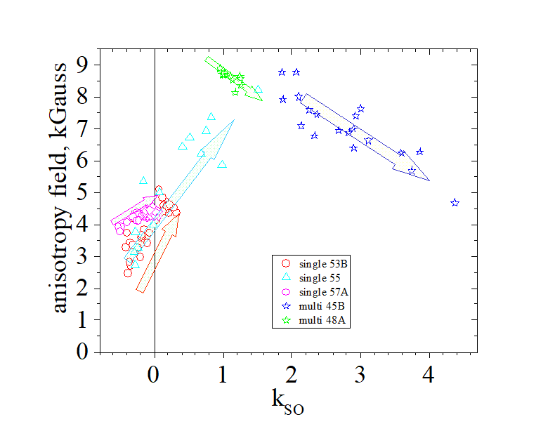
![]() (slope polarity for distribution of Hint vs. kSO) The slope is positive for single- layer nanomagnets which have a small coefficient kSO of spin- orbit interaction and large internal magnetic field Hint. The slope is negative for multi- layer nanomagnets , which have a large kSO and small Hint.
(slope polarity for distribution of Hint vs. kSO) The slope is positive for single- layer nanomagnets which have a small coefficient kSO of spin- orbit interaction and large internal magnetic field Hint. The slope is negative for multi- layer nanomagnets , which have a large kSO and small Hint.
![]()
![]()
![]() (slope polarity for distribution of Hint vs. kSO) The slope is always negative for distribution of the internal magnetic field Hint vs. kSO for both single- layer and multi- layer nanomagnets. (See Fig.44 above). It means that a smother interface always results in a larger coefficient kSO of spin- orbit interaction and a smaller the internal magnetic field Hint. The Hint is smaller because the demagnetization field becomes larger for a smoother interface.
(slope polarity for distribution of Hint vs. kSO) The slope is always negative for distribution of the internal magnetic field Hint vs. kSO for both single- layer and multi- layer nanomagnets. (See Fig.44 above). It means that a smother interface always results in a larger coefficient kSO of spin- orbit interaction and a smaller the internal magnetic field Hint. The Hint is smaller because the demagnetization field becomes larger for a smoother interface.
| Measured anisotropy field vs. measured strength of spin-orbit interaction. Systematic study. | ||||||||||||
|---|---|---|---|---|---|---|---|---|---|---|---|---|
Comparison of data of many different nanomagnets of a different size, material, composition, thickness, structure. |
||||||||||||
|
||||||||||||
| click on image to enlarge it |
![]() Why is the distribution of Hani and kSO measured for nanomagnets fabricated on one wafer important?
Why is the distribution of Hani and kSO measured for nanomagnets fabricated on one wafer important?
It is because in one wafer there are not so many variations of parameters. There is only a weak variation of interface roughness and a weak variation of the nanomagnet thickness. Other parameters remain the same. Therefore, it is easier to trace the effect of the roughness and thickness variations on parameters of a nanomagnet.
| slope of Hani vs kSO. Single-layer vs. multi-layer nanomagnets. | ||||||||||
|---|---|---|---|---|---|---|---|---|---|---|
|
||||||||||
| click on image to enlarge it |
(![]() vs.
vs. ![]() ) Why is the slope of dependence Hani vs. kSO positive for a single- ferromagnetic- layer nanomagnet, but negative for a a multi- ferromagnetic- layer nanomagnet?
) Why is the slope of dependence Hani vs. kSO positive for a single- ferromagnetic- layer nanomagnet, but negative for a a multi- ferromagnetic- layer nanomagnet?
Both the demagnetization field Hdemag and the magnetic field HSO of spin- orbit interaction are originated at an interface and, therefore, become larger when the number of interfaces increases. In a multilayer nanomagnet, the number of interfaces is larger. For this reason, both kSO and Hdemag are larger in a multilayer nanomagnet
The internal magnetic field Hint is smaller when Hdemag is larger. For a smoother interface, kSO becomes larger but Hint becomes smaller. Therefore, a positive change ΔkSO corresponds to a negative change ΔHint.
Hint is small and kSO is large in a multilayer nanomagnet. As a result, ΔHint contribution to ΔHani is large, ΔkSO contribution is small and the slope is negative (See Eq. 42.3)
Hint is large and kSO is small in a single- layer nanomagnet. As a result, ΔHint contribution to ΔHani is small, ΔkSO contribution is large and the slope is positive (See Eq. 42.3)
(![]() vs.
vs.![]() vs.
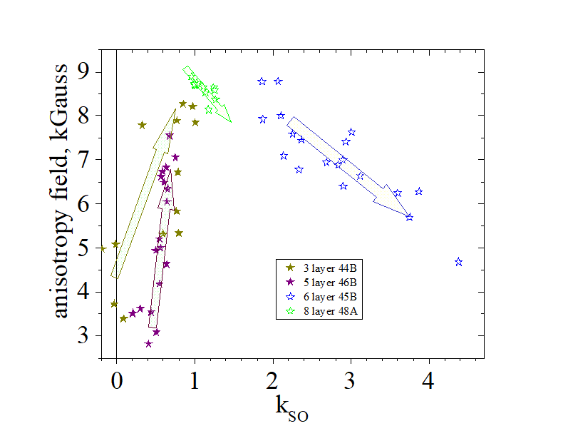
vs. ![]() ) Why is the absolute value of slope of dependence Hani vs. kSO increases at first, when number of layers increases, but starts to decreases when the number of layer exceeds some critical number?
) Why is the absolute value of slope of dependence Hani vs. kSO increases at first, when number of layers increases, but starts to decreases when the number of layer exceeds some critical number?
When the number of ferromagnetic layers increases, the interface roughness often increases as well. As a consequence, an increase of kSO and Hdemag due to the increase of the number of interface is overturned by the decrease of kSO and Hdemag due to the increase of the interface roughness.
![]()
![]()
| Effect of increase of nanomagnet thickness or interface roughness on strength of spin-orbit interaction (kSO), demagnetization field (Hdemag) , anisotropy field (Hani) and internal magnetic field (Hint) | |||||||||
|---|---|---|---|---|---|---|---|---|---|
|
|||||||||
| click on image to enlarge it |
Perfection of fabrication technology |
||||||||||||
|---|---|---|---|---|---|---|---|---|---|---|---|---|
|
||||||||||||
click on image to enlarge it |
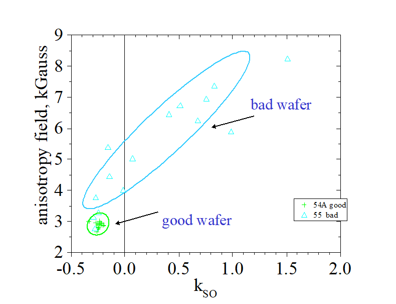
In any technological application, it is crucial to ensure uniformity among the parameters of all devices fabricated on a single wafer. This holds particularly true for nanomagnets employed in memory or sensor applications, where consistency in magnetic parameters is of utmost importance. Among these parameters, the anisotropy field and the strength of the spin-orbit interaction stand out as key factors. By measuring the distribution of the anisotropy field against the coefficient of the spin-orbit interaction, one can obtain a clear indication of the quality and precision of the underlying technology being utilized.
The measured distribution of the anisotropy field (Hani) against the coefficient (kSO) of the spin-orbit interaction serves as an indicator of the fabrication technology's quality and precision:
 (perfect fabrication technology): all data points cluster tightly within a small circle with a minimal radius.
![]() (moderate fabrication technology): although there may be some slight scattering of data points, they still align along a straight line.
(moderate fabrication technology): although there may be some slight scattering of data points, they still align along a straight line.
 (bad fabrication technology): the measured data points are noticeably sparse, dispersed over a larger area.
Evaluation of a nanomagnet fabrication technology. |
|---|
 |
A measured distribution of Hani vs. kso is a good evaluation of the fabrication technology. The case, when all data points cluster tightly within a small circle with a minimal radius, is a clear indication of perfection of the fabrication technology. |
![]() How can I determine whether the variation in roughness or the variation in thickness is responsible for the changes in magnetic properties observed in nanomagnets fabricated on a single wafer?
How can I determine whether the variation in roughness or the variation in thickness is responsible for the changes in magnetic properties observed in nanomagnets fabricated on a single wafer?
The demagnetization field does not depend on the nanomagnet thickness. As a consequence, a variation of thickness does not affect the internal magnetic field Hint, but does affect the strength of spin-orbit interaction. The distribution Hint vs. kSO along a straight horizontal line is a good indication that the variation of thickness is minimal.
It should be noted that the slope of distribution Hint vs. kSO is increases for a smaller Hint and larger kSO (See Fig 44 above)
![]() Is the distribution of the coercive field Hc for nanomagnets fabricated on the same wafer related to the distribution Hani vs. kSO?
Is the distribution of the coercive field Hc for nanomagnets fabricated on the same wafer related to the distribution Hani vs. kSO?
Yes. The coercive field Hc is related to Hani and kSO. A sparse distribution of Hani vs. kSO usually corresponds to a sparse distribution of Hc. However, there is one parameter, which may make the Hc distribution even more sparse. It is the size of the nucleation domain (see here).
The size of the nucleation domain depends very much on the smoothness, perfections and sharpness of the nanomagnet boundary, which may be very different from a nanomagnet to nanomagnet. As a consequence, a variation of size of the nucleation domain may be substantial even in the case of a reasonably good nanofabrication technology.
Dependence of strength of spin- orbit interaction on polarity of magnetic field |
||||||||||||||||||
|---|---|---|---|---|---|---|---|---|---|---|---|---|---|---|---|---|---|---|
|
||||||||||||||||||
click on image to enlarge it |
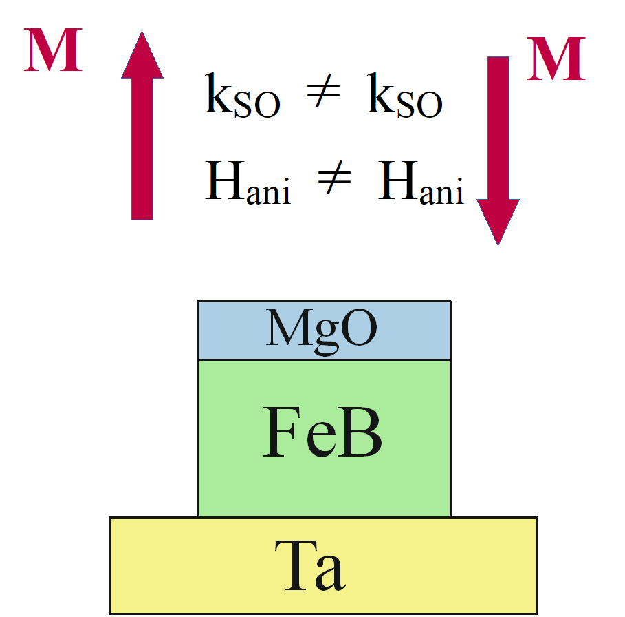
There are two stable opposite magnetization directions along the nanomagnet easy axis. Both the strength of the spin- orbit interaction and the anisotropy field are different for those opposite magnetization directions.
![]() The reason for the observed disparity is the correlation between the strength of the spin-orbit interaction and the orientation of the magnetic field relative to the orbital deformation taking place at the interface.
The reason for the observed disparity is the correlation between the strength of the spin-orbit interaction and the orientation of the magnetic field relative to the orbital deformation taking place at the interface.
![]() (demagnetization field vs. spin- orbit interaction): The demagnetization field remains unaffected by the magnetization polarity as it is solely a geometric phenomenon independent of polarity. On the other hand, the strength of the spin-orbit interaction does depend on magnetization polarity due to its reliance on the polarity of the orbital deformation with respect to the interface. Specifically, it is influenced by the direction of the orbital center's shift in relation to the nuclear position. The strength of the spin-orbit interaction varies depending on whether the magnetic field is applied in the same direction as the shift or in the opposite direction.
(demagnetization field vs. spin- orbit interaction): The demagnetization field remains unaffected by the magnetization polarity as it is solely a geometric phenomenon independent of polarity. On the other hand, the strength of the spin-orbit interaction does depend on magnetization polarity due to its reliance on the polarity of the orbital deformation with respect to the interface. Specifically, it is influenced by the direction of the orbital center's shift in relation to the nuclear position. The strength of the spin-orbit interaction varies depending on whether the magnetic field is applied in the same direction as the shift or in the opposite direction.
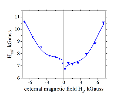
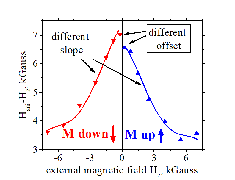
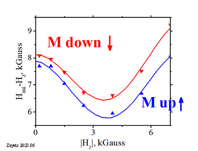
![]() (how to measure) There is a substantial difference in measured dependence of anisotropy field vs. an external magnetic field Hz, which is applied along the easy axis, for two opposite directions of Hz. Both the offset of the dependence (Hani) and the slope (kSO) are different for opposite directions of the magnetic field.
(how to measure) There is a substantial difference in measured dependence of anisotropy field vs. an external magnetic field Hz, which is applied along the easy axis, for two opposite directions of Hz. Both the offset of the dependence (Hani) and the slope (kSO) are different for opposite directions of the magnetic field.
| Measured dependences of Hani and kSO on polarity of magnetic field & magnetization | |||||||||
|---|---|---|---|---|---|---|---|---|---|
|
|||||||||
| Anisotropy field Hani vs. external magnetic field. Dots are measured data. Lines are fit. | |||||||||
| wafer VOLT 58A Ta(5 nm)/ (FeCoB 1 nm, x=0.3) (see here) nanomagnet L43C SOT | |||||||||
| click on image to enlarge it |
![]() (fact): The variation in the strength of the spin-orbit interaction in relation to magnetization reversal is a characteristic commonly found in nearly all interfaces.
(fact): The variation in the strength of the spin-orbit interaction in relation to magnetization reversal is a characteristic commonly found in nearly all interfaces.
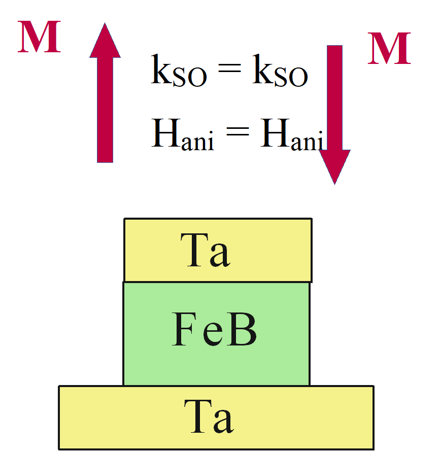
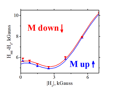
![]() What is the reason behind the lack of variation in the strength of the spin-orbit interaction during magnetization reversal for a symmetrical nanomagnet?
What is the reason behind the lack of variation in the strength of the spin-orbit interaction during magnetization reversal for a symmetrical nanomagnet?
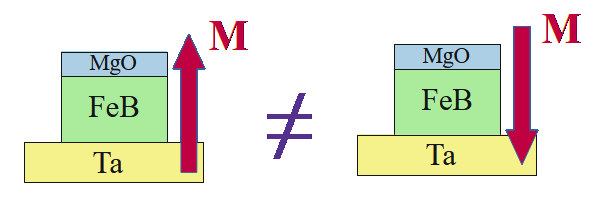
For a symmetrical nanomagnet, the absence of variation in the strength of the spin-orbit interaction with respect to magnetization reversal can be attributed to its balanced and uniform structure. There are two equal but opposite interfaces in a symmetrical nanomagnet. For example, in Ta/FeB/Ta nanomagnet there are two opposite interfaces: Ta/FeB and FeB\Ta. A variation in the strength of spin- orbit is the same, but opposite at each interface. In total, there is no variation for the symmetrical nanomagnet.
When the magnetization direction is up, the magnetic field penetrates from Ta to Fe at the lower interface and from Fe to Ta at the upper interface. When the magnetic field is reversed, there is still one interface (the upper one), where the magnetic field penetrates from Ta to Fe, there is one interface (the lower one), where the magnetic field penetrates from Fe to Ta. Even though the strength of the spin-orbit interaction is different between cases when the magnetic field penetrates from Ta to Fe and from Fe to Ta, there is no difference for the whole nanomagnet.
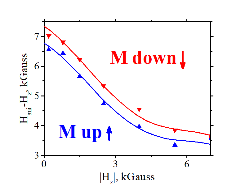
| Symmetrical vs. Asymmetrical nanomagnets | |||||||||
|---|---|---|---|---|---|---|---|---|---|
|
|||||||||
| Anisotropy field Hani vs. external magnetic field. Dots are measured data. Lines are fit. | |||||||||
| wafer VOLT 58A Ta(5 nm)/ (FeCoB 1 nm, x=0.3) (see here) nanomagnet L43C SOT | |||||||||
| click on image to enlarge it |
![]() Why does the strength of the spin- orbit interaction depend on the magnetization polarity?
Why does the strength of the spin- orbit interaction depend on the magnetization polarity?
(reason why the strength of the spin-orbit interaction increases under an external magnetic field):
The increase in the strength of the spin-orbit interaction with an increase in the external magnetic field can be attributed to the difference of orbital modifications under the influence of the Lorentz force.
The part of the orbital that rotates clockwise around the magnetic field contracts due to the Lorentz force, bringing it closer to the nucleus, where the electric field is stronger. Consequently, this portion of the orbital experiences a greater spin-orbit magnetic field.
Conversely, the counterclockwise rotating portion of the orbital expands and moves away from the nucleus, resulting in a smaller spin-orbit magnetic field.
Since the electric field diminishes with increasing distance from the nucleus following a 1/r decay, the gain from the clockwise rotating component surpasses the loss from the counterclockwise rotating component. As a result, the electron experiences an overall amplified magnetic field due to the spin-orbit interaction.

(reason why the the strength of the spin-orbit interaction depends on the polarity of an external magnetic field):
When the magnetic field is reversed, the clockwise component expands and the counterclockwise component contracts. However, due to the asymmetric nature of the orbital at the interface, the gain and loss of the spin-orbit interaction differ from the previous case. Consequently, the total gain in the magnetic field from the spin-orbit interaction varies for opposite polarities of the external magnetic field.
![]() (orbital quenching) Given that the orbital moment of localized electrons is completely quenched (see here) , resulting in a net orbital moment of zero, it raises the question of why an asymmetry exists between the clockwise and counterclockwise components of the orbital. Furthermore, what causes the interaction between the clockwise component and the up-magnetic field to differ from the interaction between the counterclockwise component and the down-magnetic field?
(orbital quenching) Given that the orbital moment of localized electrons is completely quenched (see here) , resulting in a net orbital moment of zero, it raises the question of why an asymmetry exists between the clockwise and counterclockwise components of the orbital. Furthermore, what causes the interaction between the clockwise component and the up-magnetic field to differ from the interaction between the counterclockwise component and the down-magnetic field?
Indeed, you are correct. The orbital moment of localized electrons is effectively quenched, resulting in no net orbital moment. This is achieved by the compensating contributions from the orbital components associated with electrons rotating in clockwise and counterclockwise directions. However, it is important to note that this compensation occurs for the overall orbital as a whole.
On a local scale, there can still be subtle differences. For instance, the clockwise component may be slightly shifted to the left, while the counterclockwise component may be shifted to the right due to variations in the surrounding atoms on the left and right sides of the orbital. As a result, there can be localized differences in the interaction of the clockwise and counterclockwise rotating components with an external magnetic field.
![]() (bulk vs. interface) What is the underlying reason for the significant dependence of the strength of the spin-orbit interaction on the magnetization polarity specifically at the interface, while such dependence is absent in the bulk of a ferromagnet?
(bulk vs. interface) What is the underlying reason for the significant dependence of the strength of the spin-orbit interaction on the magnetization polarity specifically at the interface, while such dependence is absent in the bulk of a ferromagnet?
For the spin-orbit interaction to exhibit a dependence on magnetization polarity, a distinct spatial symmetry of the electron orbital must be disrupted. Typically, this symmetry is broken at the interface but remains intact in the bulk of a ferromagnetic material. While local symmetry breaking can occur, on average, the symmetry is maintained within the bulk.
The bulk of the ferromagnetic material resembles a multilayer nanomagnet, where each interface breaks the symmetry, but subsequent interfaces exhibit equal and opposite symmetry breaking. As a result, the overall symmetry remains unbroken.
![]() (neighboring orbitals) Does the contraction or expansion of an electron's orbital under the influence of the Lorentz force take into account the neighboring orbitals of other localized electrons surrounding it?
(neighboring orbitals) Does the contraction or expansion of an electron's orbital under the influence of the Lorentz force take into account the neighboring orbitals of other localized electrons surrounding it?
Indeed, the orbital of a localized electron forms strong bonds with the orbitals of neighboring atoms. Because of the strong bonding, the strength of these bonds remains unaltered under the influence of an external magnetic field. However, within the context of unchanged overall bonding strength, there is a redistribution of the clockwise and counterclockwise rotation components of the orbital, which helps to break the required spatial symmetry.
The presence of neighboring orbitals plays a significant role in breaking the required spatial symmetry. For instance, when different atoms are situated on each side of the orbital, the center of the orbital becomes shifted away from the nucleus position. Furthermore, such neighboring orbitals make the clockwise and counterclockwise rotation components of the orbital experience shifts in different directions, thereby breaking the symmetry between them. As a result, the interaction of the clockwise and counterclockwise rotating components with an external magnetic field becomes different.
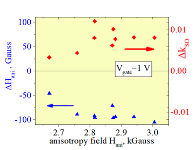
 Distribution of a change of Hani vs. a change of kso under magnetization reversal
The anisotropy field (Hani) and the coefficient of spin-orbit interaction (kSO) both exhibit a dependence on the magnetization polarity. These dependencies are not independent but are correlated with each other. Specifically, a larger change in kSO corresponds to a smaller change in Hani when the magnetization is reversed.
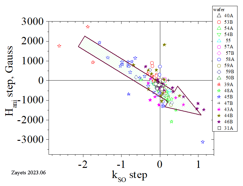
| Change of anisotropy field and strength of spin- orbit interaction under magnetization reversal. |
|---|
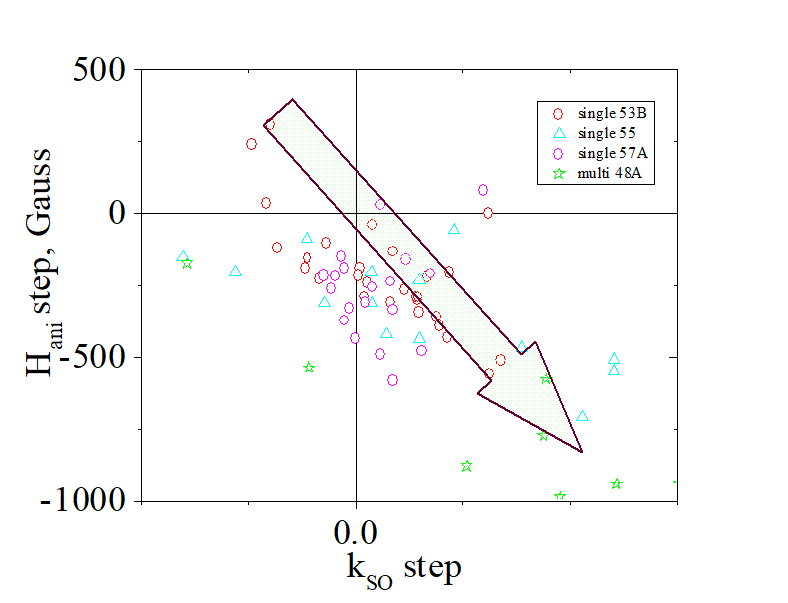 |
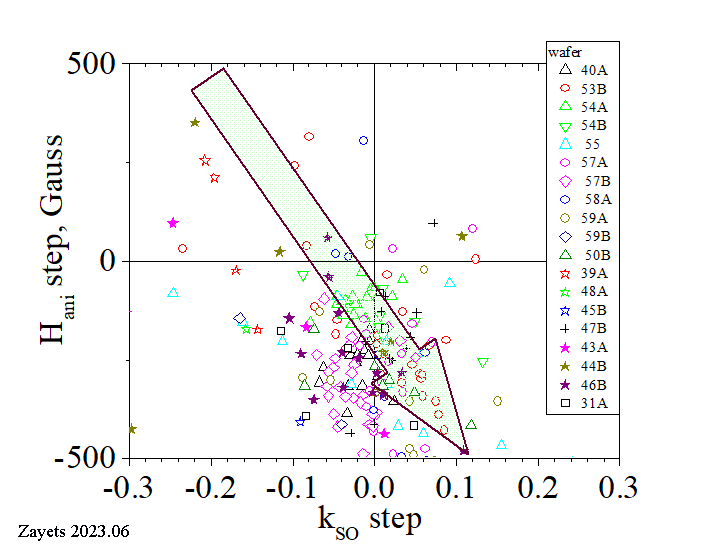
| Each dots corresponds to a measurement of one nanomagnet. Dots of the same shape and color correspond to nanomagnets fabricated on the same wafer. |
| A negative slope is very clear. A nanomagnet, which have a larger step of kso, has a smaller step of Hani. |
| click on image to enlarge it |
| What is the explanation for the negative slope observed in the distribution of the change in anisotropy field versus the change in the strength of the spin-orbit interaction under a reversal of magnetization? |
|---|
 |
| The distinction in the strength of the spin-orbit interaction during magnetization reversal is evident, but it is expected that the demagnetization field remains unaffected as it is purely a geometrical phenomenon. Consequently, one would anticipate a positive slope in the distribution. However, experimental observations reveal a negative slope. The question then arises: why is this the case? |
| As 2023.06, the reason for the experimentally- observed negative slope of distribution ΔHani vs. ΔkSO is not understood. |
This correlation becomes evident when comparing measurement data from nanomagnets fabricated on the same wafer. Within a single wafer, there are slight variations in thickness and interface roughness from point to point. Consequently, nanomagnets fabricated at different locations, such as the center or edge of the wafer, or even neighboring points, will exhibit variations in their parameters due to differences in interface roughness and nanomagnet thickness.
![]() (fact) The strength of spin-orbit interaction and, therefore, kSO does depend on the magnetization polarity
(fact) The strength of spin-orbit interaction and, therefore, kSO does depend on the magnetization polarity
It is because the position of the center of the electron orbital with respect to the nucleus position is shifted towards (outwards) the interface. The magnetic field opposite or along that shift induces a different strength of spin- orbit interaction.
![]() (fact) The demagnetization field does not depend on the magnetization polarity
(fact) The demagnetization field does not depend on the magnetization polarity
It is The demagnetization is a geometrical effect. There is any reason why the demagnetization filed should depend on the magnetization polarity.
![]() (unexplained experimental fact): negative slope between a change of kSO vs change of Hani under magnetization reversal
(unexplained experimental fact): negative slope between a change of kSO vs change of Hani under magnetization reversal
Hani is proportional to kSO and the internal magnetic field Hint:
![]()
Since the demagnetization field remains unaffected by changes in magnetization polarity, the internal magnetic field Hint: should be independent of the magnetization polarity as well. Therefore, one would expect the change in anisotropy field with magnetization reversal to have the same polarity as the change in kso. However, contrary to these expectations, the observed polarity in experiments is opposite.
![]() (A possible reason): dependence of demagnetization field on the magnetization polarity
(A possible reason): dependence of demagnetization field on the magnetization polarity
But why and how? What is the mechanism?
The negative slope is a systematic feature, which is observed in all studied wafer
Change of anisotropy field and strength of spin- orbit interaction under magnetization reversal. Systematic study. |
||||||||||||
|---|---|---|---|---|---|---|---|---|---|---|---|---|
Comparison of data of many different nanomagnets of a different size, material, composition, thickness, structure. |
||||||||||||
|
||||||||||||
| click on image to enlarge it |
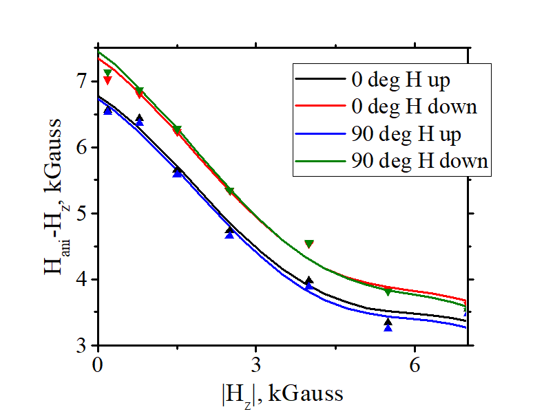
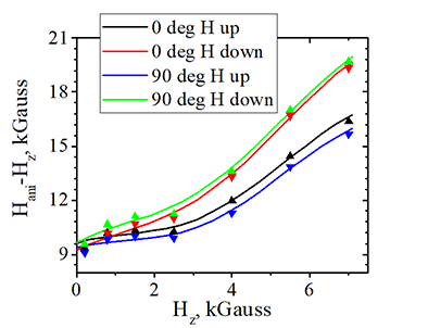
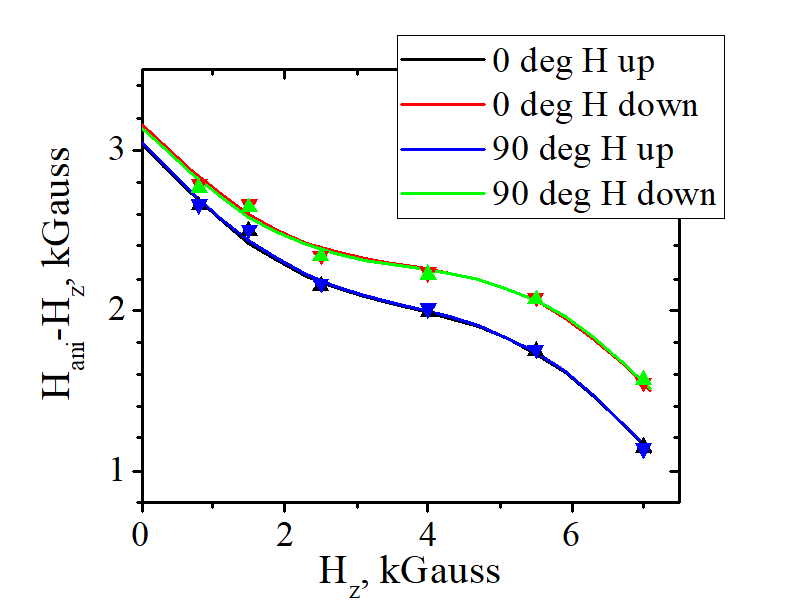
| Measured dependences of Hani and kSO on polarity of magnetic field & magnetization | |||||||||
|---|---|---|---|---|---|---|---|---|---|
|
|||||||||
| Anisotropy field Hani vs. external magnetic field. Dots are measured data. Lines are fit. | |||||||||
| Measurement of 0 deg corresponds to a scan of in-plane magnetic field along current. Measurement of 90 deg corresponds to a scan of in-plane magnetic field perpendicularly to the electrical current. Independent measurements give the same difference of the offset (Hani) and slope (kSO) | |||||||||
| (note) In all shown nanomagnets, the split due to magnetization reversal is identical for the 0-deg and 90-deg scans. It is not always the case. | |||||||||
| click on image to enlarge it |

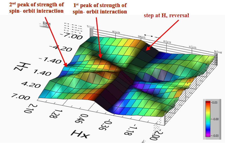
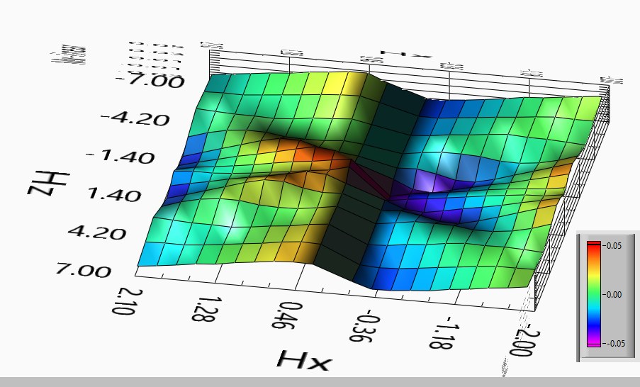
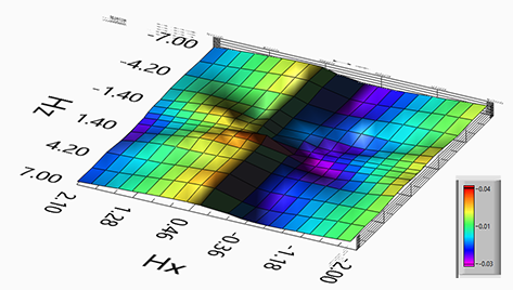
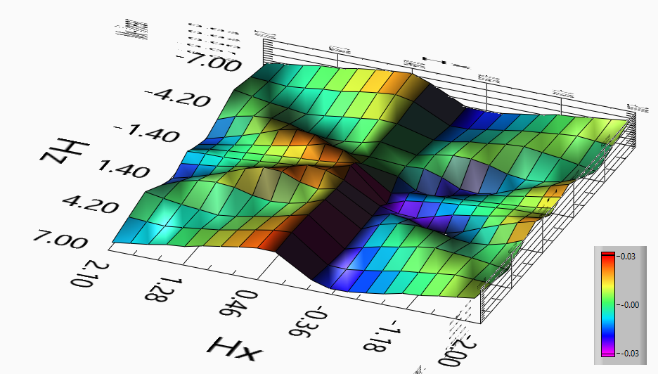
The strength of spin-orbit interaction relies on the relative angle between the magnetization and the magnetic easy axis or the surface normal for a nanomagnet with PMA. At particular angles, there exists a peak or a trough in the strength of the spin-orbit interaction. This specific angle corresponds to characteristics related to the distortion of electron orbitals resulting from bonding at the nanomagnet's interface. Across all nanomagnets examined, a consistent and systematic correlation was observed between the magnetization angle and the spin-orbit interaction.
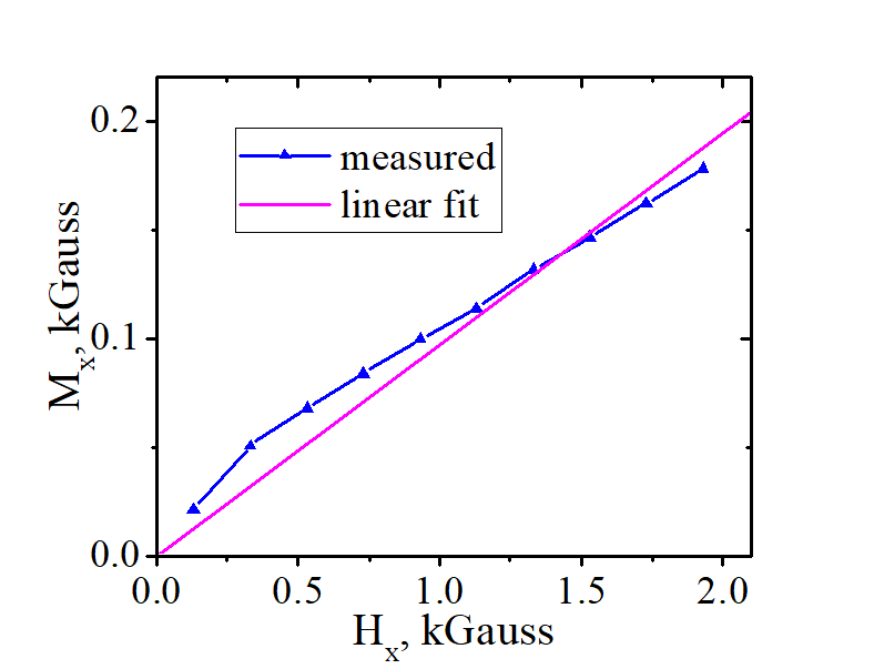
In addition to the prominent linear relationship between Mx and Hx, which serves as the basis for assessing the strength of spin-orbit interaction , there exists a secondary weak oscillatory dependence on the tilting angle. This weak oscillating pattern allows for the evaluation of the angle dependency of the spin-orbit interaction.
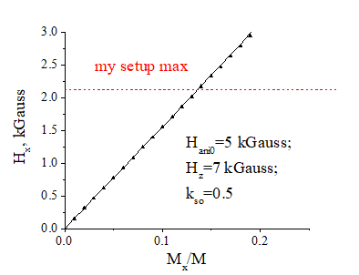
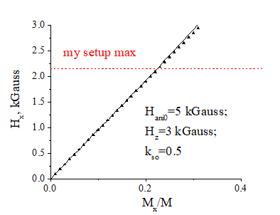
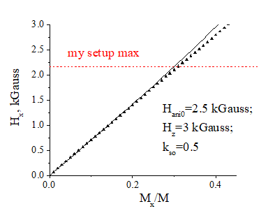
Major prominent linear relationship between Mx and Hx, from which the strength of the spin orbit interaction is evaluated,:
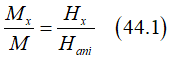
where Mx is in-plane component of the magnetization, Hx is in-plane external magnetic field and Hani is the anisotropy field , which is evaluated from the linear fitting of measured data of Mx vs. Hx.
Real measured dependency between Mx and Hx,
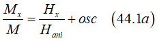
where osc is a very weak oscillations.
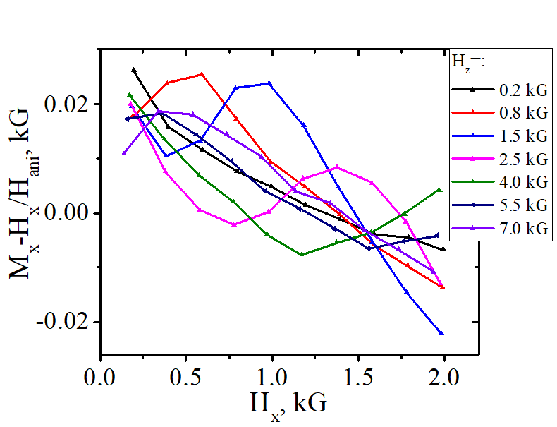
| measured dependency Mx vs. Hx, & its linear fit | Deviation of measured Mx vs. Hx from linear Relationships Mx-Hx/Hani |
|
|---|---|---|
 |
 |
 |
| wafer Volt40A nanomagnet L43C |
 |
 |
 |
| wafer Volt54A nanomagnet R65C | wafer Volt58A nanomagnet L23C | wafer Volt40A nanomagnet L43C |
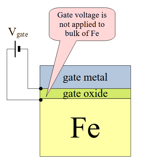
voltage-controlled magnetic anisotropy. VCMA effect. |
||||
| The VCMA effect describes the modulation of the magnetic properties of ferromagnetic metal by a gate voltage | ||||
|
||||
| click on image to enlarge it |
There is a screening of the gate voltage in the bulk of the nanomagnet. Even though the gate voltage is applied to the nanomagnet, in fact, due to the screening the gate voltage is only applied to the interface and, therefore, modulation of magnetic properties of the interface by the gate voltage is the key effect here.
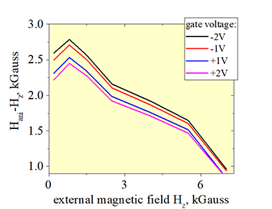
| Change of strength of spin- orbit interaction and anisotropy field under a gate voltage | |||||||||||||||
|---|---|---|---|---|---|---|---|---|---|---|---|---|---|---|---|
|
|||||||||||||||
| wafer Volt 54a (see here), nanomagnet L25C | |||||||||||||||
| click on image to enlarge it |
The magnetic anisotropy itself is originated by the spin-orbit interaction. In absence of the spin- orbit interaction there is no magnetic anisotropy and the anisotropy field Hani equals zero. It is plausible to assume that an increase of the strength of the spin- orbit interaction always leads to an increase of the anisotropy field. Often it is true. However, sometimes the dependency is opposite, an increase of the strength of the spin- orbit interaction is accompanied by an decrease of the anisotropy field, when some of nanomagnet parameters changes. It is because additionally there are changes of the demagnetization field and the internal magnetic field, which can be opposite to the change of the spin-orbit interaction and which can reverse the change of Hani.
![]()
![]()
.
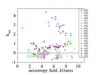
Systematic measurements in FeCoB nanomagnets of a different structure and composition |
|||||||||||||||||||||
|---|---|---|---|---|---|---|---|---|---|---|---|---|---|---|---|---|---|---|---|---|---|
dependence on anisotropy field Hani |
|||||||||||||||||||||
|
|||||||||||||||||||||
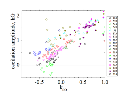
dependence on strength of spin-orbit interaction kSO |
|||||||||||||||||||||
|
|||||||||||||||||||||
| Dots of the same color and shape correspond to nanomagnet fabricated at different places of the same wafer. Stars show multilayer nanomagnets, which contain several ferromagnetic layers. | |||||||||||||||||||||
| click on image to enlarge it |
Strength of spin-orbit interaction is largest in multilayer nanomagnets, which are shown by stars and which contain several ferromagnetic layers. There is a linear dependence between kSO vs. Hani. In case of a single- layer nanomagnet, the slope of the linear dependence is positive. In case of a multi- layer nanomagnet, the slope is negative.
A. (2024.03) Quantifying individual contributions to the strength of spin-orbit interaction from the bulk and the interface of the nanomagnet is a challenging task, albeit potentially feasible. The measured data (See Fig. above) presents a qualitative assessment, derived from the clear observation that the strength of spin-orbit interaction increases with the number of interfaces, along with the negative kso systematically measured for thick single-layer nanomagnets with predominant bulk contribution.
As demonstrated above (see here) , a negative value of kso indicates that while all elements of the tensor of spin-orbit interaction remain positive, the spin-orbit interaction is greater in the in-plane direction than in the perpendicular-to-plane direction.
The challenge of separating bulk and interface contributions arises from the significant influence of interface roughness on spin-orbit interaction, compounded by difficulties in maintaining uniformity of interface roughness across nanomagnets of varying thicknesses.
A. (2024.03) The atomic environment surrounding Fe and Co atoms differs significantly at the interface compared to the bulk. In the bulk, Fe atoms are surrounded only by other Fe atoms, resulting in nearly isotropic spin-orbit interaction. However, at the interface, the surrounding atoms differ above and below the Fe atoms, leading to asymmetric forces experienced by the atom from different directions, which leads to an orbital deformation in comparison with a bulk Fe atom.
As depicted in Fig. (see above), the measured value of kso for single-layer nanomagnets with a larger bulk contribution is close to 0, indicating that the strength of spin-orbit interaction is nearly equal in all directions. In contrast, kso approaches a value of 9 for multilayer nanomagnets, where the interface contribution is predominant. This suggests that at the interface, where Fe atoms are subject to deformation, the spin-orbit interaction is significantly stronger in the perpendicular-to-plane direction than in the in-plane direction.
A. (2024.03) Due to its relativistic nature, the spin-orbit interaction manifests itself only when the time-reversal symmetry (T-symmetry) of an electron orbital is broken. However, the spin-orbit interaction itself cannot break the T-symmetry—it necessitates an external T-symmetry-breaking factor. This only occurs when the electron is subjected to conditions where T-symmetry is already broken. There are a limited number of scenarios where this occurs: (1) in the presence of an electrical current, (2) when the electron possesses a nonzero orbital moment due to its non-quenched state, and (3) when an external magnetic field is applied. It's noteworthy that the intrinsic magnetic field within a ferromagnetic or antiferromagnetic material is regarded as an external field. Consequently, the necessity of a broken T-symmetry for the spin-orbit interaction's existence already clarifies why its strength is proportional to the external magnetic field.
While slightly oversimplified, the following provides a very illustrative explanation: Consider a fully quenched electron orbital under an external field. This scenario closely resembles the behavior of a localized d- electron in materials such as Fe or Co, which are nearly fully quenched, as indicated by FMR (Ferromagnetic Resonance). Full quenching implies that the orbital moment is zero, and the electron wavefunction can be divided into two components corresponding to clockwise and counterclockwise movements. In the absence of the orbital moment and external magnetic field, these two components experience equal but opposite magnetic fields of spin-orbit interaction due to the electrical field of the nucleus. Consequently, these contributions balance each other, resulting in the electron experiencing no net spin-orbit interaction. This is the case when T-symmetry is unbroken for the orbital movement. Reversing the flow direction of time implies an exchange between clockwise and counterclockwise movement paths, which, in this case, doesn't alter anything. For spin-orbit interaction to exist, there must be a distinction between clockwise and counterclockwise rotations, indicating the breaking of T-symmetry. This symmetry can be externally broken by applying a magnetic field, which creates the Lorentz force. The Lorentz force affects the electron differently along its clockwise and counterclockwise paths. The force pushes the clockwise-rotating part of the electron wavefunction away from the nucleus while drawing the counterclockwise-rotating part closer to it. This creates a disparity in the electric field of nucleus experienced by the electron for these two opposite rotations. As a result, the equilibrium between opposing magnetic fields of spin-orbit interaction is disrupted, leading to a significant magnetic field of spin- orbit interaction experienced by the electron.
The linear relationship between the strength of the spin-orbit interaction and the external magnetic field is rooted in the relativistic nature of spin-orbit interaction and, importantly, in the fundamental features of broken time-reversal symmetry (T-symmetry). Due to its relativistic origin, the spin-orbit interaction occurs only when T-symmetry is externally broken. It's crucial to note that spin-orbit interaction cannot break T-symmetry by itself.
Depending on the source of the T-symmetry breaking, there are three distinct types of spin-orbit interaction. For the first type, T-symmetry is broken by an electrical current, as seen in phenomena like the Spin Hall effect. For the second type, occurring in unquenched electrons, T-symmetry is broken due to the orbital moment (e.g., alignment of spin and orbital moments in an atomic gas). For the third type, which is responsible for magnetic anisotropy, T-symmetry is broken by a magnetic field.
Since there is no spin-orbit interaction in the absence of a magnetic field H, and the polarity of Hso follows the polarity of H, Hso should be an odd function of H, meaning it should be proportional to the 1st, 3rd, 5th orders of H. Experimental evidence clearly indicates that the linear component is the largest, while other components are negligible, at least in the case of classical ferromagnetic metals like Fe and Co.
A. (2024.03) The spin-orbit interaction exists only when the time-inverse symmetry (T-symmetry) is broken. There are three very different types of spin-orbit interaction, each corresponding to a distinct method of breaking T-symmetry. The features and properties of each type of spin-orbit interaction are drastically different, necessitating the assignment of a unique designation to each type to avoid possible confusion.
The interaction between the magnetic field of spin-orbit interaction and electron spins results in different energies for light-hole, heavy-hole, and split-off bands for valence electrons in a semiconductor. The second way to break T-symmetry is due to the flow of an electrical current. This type of spin-orbit interaction is responsible for the existence of the whole family of magneto-transport effects (the Spin Hall effect, AHE, AMR/PHE effect and so on). These effects arise from spin-dependent scatterings. The scatterings become spin- dependent because of spin-orbit interaction, resulting in the breaking of T-symmetry by the electrical current. The third way to break T-symmetry is by applying an external magnetic field. This type of spin-orbit interaction is responsible for magnetization alignment in a magnet and for magnetic anisotropy. Only the measurement of the last type of spin- orbit interaction is described above.
All references you mentioned pertain to magneto-transport effects, which are associated with the second type of spin-orbit interaction.
A. (2025.03) I agree with you that the spin- orbit interaction varies significantly among different electrons. In particular, the type, origin, and strength of SOI differ substantially between conduction and localized electrons. For conduction electrons, a nonzero orbital moment plays a key role in their spin-orbit interaction, whereas for localized electrons—despite their nearly quenched orbital moment, so their orbital moment is nearly zero—SOI remains one of the strongest among all electrons in a solid due to a different underlying mechanism. This distinction is evident in the behavior of the g-factor: for conduction electrons, it varies widely, ranging from negative to large positive values, while for localized electrons, it remains close to 2, as consistently observed in ferromagnetic resonance (FMR) measurements.
The fundamental reason for these differences is that SOI manifests only when time-reversal symmetry (T-symmetry) is broken by an external factor. The specific mechanism of T-symmetry breaking defines the nature of the spin-orbit interaction. Three primary types of SOI can be distinguished: The first type of spin-orbit interaction arises when there is an unquenched orbital moment, commonly observed in conduction electrons and orbital electrons within atomic gases. The second method of breaking T-symmetry involves the application of an external magnetic field. This type of spin-orbit interaction is induced by an external magnetic field and exhibits a linear relationship with the externally applied magnetic field. The third type of spin-orbit interaction emerges in the presence of an electrical current, which breaks the T-symmetry. This type of spin-orbit interaction leads to a dependency of scattering probabilities of conduction electrons on their spin direction.
A. (2025.03) The spin-orbit interaction (SOI) that governs transport phenomena—such as the Anomalous Hall effect, Spin Hall effect, Inverse Spin Hall effect, and Anisotropic Magnetoresistance/Planar Hall effect—is fundamentally different from the SOI of localized electrons responsible for perpendicular magnetic anisotropy (PMA).
While the primary origin of both effects is the same: both effects originate from the relativistic motion of electrons around the nucleus, they differ due to the distinct mechanisms that break time-reversal symmetry (T-symmetry). In magneto-transport phenomena, T-symmetry is broken by an electrical current, leading to spin-dependent scattering. In contrast, for magnetic anisotropy in ferromagnetic nanomagnets, T-symmetry is broken by the internal magnetic field within the ferromagnetic material.
Because these are distinct manifestations of SOI, the effective spin-orbit coupling constants derived from transport measurements (e.g., low-temperature spectroscopy or absorption or the family of magneto-transport effects) cannot be directly compared to those extracted from measurements of magnetic anisotropy. The SOI strength in transport effects reflects spin-dependent scattering mechanisms in conduction electrons, whereas the SOI strength in interfacial PMA describes the interaction of localized electrons with the internal magnetic field influenced by orbital deformation at interface with addition influence of the demagnetization field. Thus, these two effects inherently have different characteristic SOI parameters.
The term Hanis=Hz in the equation corresponds to the bulk contribution, representing the alignment of magnetization along the total magnetic field in vacuum, which doesn't provide informative insights. Consequently, when conducting data analysis, it is more advantageous to utilize the relationship between Hanis-Hz , and Hz. This approach ensures that the significant bulk contribution does not obscure a potentially weaker dependence on kso.
Please see this figure here
The experiment is performed at a high magnetic field higher than 1 kGauss, at which magnetic domains do not exist. Additionally, nanomagnets are specifically utilized due to their lack of magnetic domains, simplifying data analysis. However, this measurement method allows for its application to larger samples without significant issues.
The presence and impact of magnetic domains under a weak magnetic field can be easily identified in this measurements, and their influence can be removed by a slight increase in the magnetic field.
This trend is highly systematic. For all studied nanomagnets, kso consistently exhibits a large and positive value in multilayer nanomagnets. In contrast, for single-layer nanomagnets, kso is always small and can be either positive or negative.
A negative value of kso indicates that the strength of the spin-orbit interaction in the in-plane direction is greater than in the perpendicular-plane direction . Generally, the interface kso contribution is positive, while the bulk kso contribution is often negative.
In FeB and FeCoB amorphous nanomagnets, the major contribution to kso originates from interfaces, which is positive and accumulates with an increasing number of interfaces. This is why kso is large in multilayer nanomagnets. However, the strength of the spin-orbit interaction strongly depends on interface imperfections, such as roughness and sharpness. An increase in the number of interfaces leads to an increase in interface imperfections, which eventually causes a decrease in kso after a certain number of interfaces. Therefore, precise fabrication is key to achieving a large positive kso.
(variation of kso between positive and negative values) The interface kso contribution is positive, while the bulk kso contribution is often negative. The sign of kso is determined by the balance between these contributions. In thicker nanomagnets, the bulk contribution predominates, resulting in a negative kso. Conversely, in thinner nanomagnets, the interface contribution is dominant, leading to a positive kso
(variation of kso for a different nanomagnets fabricated on the same wafer): A variation in kso was observed among the data points of nanomagnets fabricated at different locations on the same wafer. It was noted that the closer two nanomagnets are to each other, the smaller the differences in kso tend to be. A more homogeneous and smoother wafer corresponds to reduced kso variation. This spread in data serves as an indicator of the precision of the fabrication technology. Both variations in thickness and surface roughness contribute to data dispersion on a wafer. Given that nanomagnet thickness is around 1 nm, even a variance within the range of a single atomic layer can markedly impact kso. Moreover, it was experimentally observed in this work that the surface roughness and the surface sharpness play an even more substantial role, exerting a notable influence on kso.
The large value of kso is common in multilayer nanomagnets. In FeB and FeCoB amorphous nanomagnets, the major contribution to kso originates from interfaces, and this contribution accumulates with an increasing number of interfaces. This is why kso is large in multilayer nanomagnets. However, the strength of the spin-orbit interaction strongly depends on interface imperfections, such as roughness and sharpness. An increase in the number of interfaces leads to an increase in interface imperfections, which eventually causes a decrease in kso after a certain number of interfaces. Therefore, precise fabrication is key to achieving a large kso.
My current fabrication technology is good and I am able to fabricate nanomagnets with a large kso, but I believe that using more advanced fabrication technologies could yield even higher values of kso.
I completely agree with you. When the scanning field is close to the anisotropy field, the approximation (Mx/M) ^2<<1 (Eq.A11 of AIP Advances (2024)) is no longer valid, and the relationship between Mx and Hx becomes non-linear. However, this limitation does not pose any issues in my measurements for the following reasons:
(reason 1) : Direct Calculation:
It is entirely feasible to calculate the anisotropy field Hani directly from the non-linear relationship between Mx and Hx without relying on any approximations, including Eq. A11 of AIP Advances (2024). Therefore, Hani can be evaluated from experimental data by a non-linear fitting without risking any error.
(reason 2) : Validity of Approximation:
For realistic parameters of FeCoB nanomagnets and the maximum magnetic field provided by my magneto-transport probe, the condition (Mx/M) ^2<<1 (Eq.A11) strictly holds for all the nanomagnets I have studied.
These factors ensure that the validity of the approximation does not introduce any complications in the interpretation or accuracy of the results.
![]() (reason 1) (Calculation of explicit equation for relation between Hx and Mx):
(reason 1) (Calculation of explicit equation for relation between Hx and Mx):
The implicit non-linear relation between Mx and Hx was calculated in Appendix A of AIP Advances (2024) as
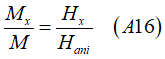
where
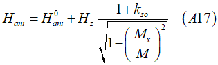
From Eq. (A17), the explicit non-linear equation for relation between Hx vs Mx is calculated as
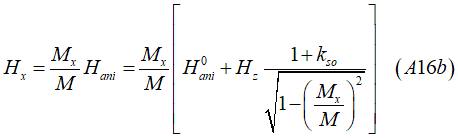
A non-linear fitting of the experimentally measured Mx vs.Hx data using Eq. A16b is employed to determine Hani. Prior to this, a linear fitting is performed to estimate an initial approximation of Hani and kso. These calculations are integrated into a program, which I specifically designed for analyzing the experimental data.
![]() (reason 2) (Validity of Approximation (Mx/M) ^2<<1 (Eq.A11 of AIP Advances (2024)) for my samples + my probe limitations):
(reason 2) (Validity of Approximation (Mx/M) ^2<<1 (Eq.A11 of AIP Advances (2024)) for my samples + my probe limitations):
Although I have the option to perform a non-linear data analysis without relying on any approximations, I generally prefer linear data analysis. This preference arises because the difference between the results of the two methods is negligibly small, and linear analysis is more robust in the presence of additional oscillations in the data.
It is also worth noting that the maximum in-plane magnetic field generated by my probe is 2.2 kGauss, whereas the measured anisotropy fields of FeCoB nanomagnets under Hz are substantially larger, ranging from 5 to 30 kGauss. This ensures that the measurements are conducted well within the relevant field range for these nanomagnets.
Below graphs compare non- linear calculation (solid line, no approximations) with linear calculation (dot line) for most extreme possible cases of measurements. You can see that in all cases the difference is negligible. A tiny difference appears only in the unrealistic case of a very small Hani=2.5 kGauss. It is worth notice that coercive field of a nanomagnet with Hani=2.5 kGauss (Hz=0) is extremely small (Hc<10 Gauss) and which magnetization experiences the spontaneous telegraphic switches
| Correctness of linear approximation of relation Mx vs.Hx | |||
|---|---|---|---|
|
|||
| dot line: linear approximation, solid line: no approximations | |||
| Mx: the component of magnetization perpendicular to the easy axis; Hx: magnetic field applied perpendicular to the easy axis |
A. (2024.03) As a result of interface roughness, the positions of neighboring atoms undergo slight variations, causing subtle changes in orbital deformation. Consequently, this variance leads to fluctuations in the strength of the spin-orbit interaction across different local nanomagnets fabricated at different local positions.
Figure (see above) provides a distinct experimental validation of this phenomenon. Keeping other nanomagnet properties constant, a higher kso value signifies a smoother and sharper interface.
A. (2024.03) The impact of surface roughness on demagnetization and, consequently, on magnetic anisotropy is an established experimental observation. In addition to the evidence provided in Fig. 2, there are two more experimental validations. The specifics of the measured modulation of the strength of spin-orbit interaction by a gate voltage (VCMA effect) and by an electrical current (SOT effect) distinctly indicate the significance of influence of surface roughness on demagnetization and the important role of this influence on observed features of those two effects. Detailed data from these measurements will be published in another manuscript and were presented and discussed at the last Intermag conference.
The reason behind the reduction in demagnetization field with increasing surface roughness is straightforward. It is a known fact that the demagnetization field is larger for a smooth plane than for a sphere. A rough surface can be conceptualized as a plane surface covered by spheres. Since each sphere reduces the demagnetization field, the overall demagnetization field of such a rough surface is smaller compared to that of a perfectly smooth surface. Moreover, as the surface becomes rougher, the spheres protrude further from the surface, further reducing the demagnetization field.
A. (2024.03) The demagnetization field represents the magnetic field of a sequence of the magnetic dipoles, interrupted by the interface. In the scenario of a perfectly smooth surface, this magnetic field aligns precisely along the surface normal at every point. However, in the presence of surface roughness, deviations from the surface normal occur, and these deviations vary slightly across the surface. When averaged, the direction of the demagnetization field remains aligned with the surface normal, but its magnitude reduces. Consequently, the demagnetization field is larger for a smoother surface.
The observed oscillations represent unique and unexpected features of the spin-orbit interaction. I am confident that in the future, detailed theoretical and experimental studies will be conducted to explore these intriguing oscillations further. For these forthcoming investigations, the primary linear background can be subtracted to highlight and analyze the oscillatory behavior. However, for the current study, it is imperative to emphasize the main linear dependence as the key finding.
The origin of the observed oscillations in the strength of the spin-orbit interaction remains unknown. One plausible explanation is that the changing distribution of electron orbitals under an external magnetic field is influenced by the different energy levels of neighboring atoms making a slight oscillating variation in the strength of the spin- orbit interaction.
Furthermore, the strength of the spin-orbit interaction is significantly affected by the roughness and sharpness of the interface, as evidenced by clear experimental observations. This implies that the strength of the spin-orbit interaction is highly dependent on the precise positions of atoms at the interface. As the roughness varies slightly from one nanomagnet to another, so does the distribution of atoms at the interface. Therefore, if the oscillations are indeed caused by the influence of neighboring atoms, their amplitude should also vary from one nanomagnet to another.
A. (2024.03) At present, the origin of the oscillations remains unknown. It is clear that this intriguing phenomenon lacks a simple explanation and deserves further investigation through both theoretical and experimental studies.
One plausible explanation is that the changing distribution of electron orbitals under an external magnetic field is influenced by the different energy levels of neighboring atoms making a slight oscillating variation in the strength of the spin- orbit interaction.
Furthermore, the strength of the spin-orbit interaction is significantly affected by the roughness and sharpness of the interface, as evidenced by clear experimental observations. This implies that the strength of the spin-orbit interaction is highly dependent on the precise positions of atoms at the interface. As the roughness varies slightly from one nanomagnet to another, so does the distribution of atoms at the interface. Therefore, if the oscillations are indeed caused by the influence of neighboring atoms, their amplitude should also vary from one nanomagnet to another. That tendency aligns precisely with experimental data depicted in Figure (See above).
The observed oscillations exhibit consistent and systematic behavior across all studied nanomagnets. The oscillation amplitude, period, and phase were obtained by fitting the experimental data to a linear function with superimposed oscillations. The evaluated oscillation period and phase were nearly the same for all samples, varying within a narrow range.
The oscillations are clearly an interfacial feature of the spin-orbit interaction, as their amplitude is largest in thinner nanomagnets, where the interfacial contribution dominates, and smallest in thicker nanomagnets, where the bulk contribution predominates.
Conservation of T-symmetry requires that the magnetic field of spin- orbit interaction Hso be an odd function with respect to the external magnetic field Hext. Experimental measurements show that the dependence of Hso on Hext exhibits an approximately linear trend with minor oscillations superimposed. While there should be components proportional to H^3 and H^5, these are small and difficult to detect compared to the dominant linear component. The oscillations are clearly an interfacial feature of the spin-orbit interaction, as their amplitude is largest in thinner nanomagnets, where the interfacial contribution dominates, and smallest in thicker nanomagnets, where the bulk contribution dominates.
(possible origin of oscillations) The spin-orbit interaction depends on the shape of the orbital because it determines the degree and specifics of how the external magnetic field breaks the T-symmetry of the orbital. At the interface, the orbital shape is complex and influenced by atoms of two different materials on both sides of the interface. Although the exact origin of the oscillations is still unknown, it can be inferred that such a complex interaction may exhibit some oscillatory behavior.
The observed effect cannot be attributed to coercivity or hysteresis for several reasons. First, all measurements were conducted under a bias magnetic field Hz ranging from 0.8 kG to 7 kG, which is substantially larger than the coercive fields of the studied FeCoB nanomagnets (20 G to 450 G). Prior to each measurement, the magnetization was fully reversed under a magnetic field of 7 kG, ensuring that the system was well beyond any coercive effects. Second, nearly all the nanomagnets studied are of the single-domain type. These structures lack subdomains even under small magnetic fields or in the absence of a magnetic field, eliminating any contribution from domain-related hysteretic behavior. Thus, the difference in kso and Hani between positive and negative Hz cannot be explained by coercivity or hysteresis but must arise from other intrinsic factors of the system.
The dependency of strength of the spin- orbit interaction on the magnetization direction is not surprising, common and important for the existence of many magnetostatic effects. For example, this dependency is a critical factor for the existence of magnetic anisotropy. Without such a directional dependence, perpendicular magnetic anisotropy (PMA) would not be observed in amorphous nanomagnets. Another key factor influencing magnetic anisotropy is the demagnetization field, which is maximal for perpendicular-to-plane magnetization and nearly absent for in-plane magnetization. In the case of an isotropic spin-orbit interaction, the easy axis and equilibrium magnetization of any nanomagnets is always in-plane. Only when the spin-orbit interaction is stronger in the perpendicular-to-plane direction, the direction of easy axis and equilibrium magnetization can become perpendicular to the plane.
The PMA in FeCoB nanomagnets is known to have an interfacial origin. The directional dependence of spin-orbit interaction for Fe atoms located either in the bulk or at interface has been measured independently (see my AIP2024 paper here). For Fe atoms at the interface, the spin-orbit interaction is significantly stronger in the perpendicular-to-plane direction, while for bulk Fe atoms, it is nearly isotropic, with a slight preference for in-plane directions. Detailed theoretical explanations and calculations of how and why this directional dependence influences magnetic anisotropy are provided in Appendix A of my AIP2024 paper
This directional dependence can also be understood qualitatively. In the bulk of an amorphous nanomagnet, Fe atoms have symmetrical surroundings, resulting in symmetric orbitals and nearly isotropic spin-orbit interaction. At the interface, however, the d-electron orbitals of Fe atoms experience asymmetrical interactions due to the different atomic environments above and below the interface. For example, in Fe/MgO, the Fe orbitals are more strongly influenced by oxygen atoms above than by Fe atoms in the bulk below, leading to a directional asymmetry in spin-orbit interaction strength. This asymmetry explains why the interaction strength differs for in-plane and perpendicular-to-plane magnetization directions.
Similarly, the difference in spin-orbit interaction strength for opposite magnetization directions can also be qualitatively attributed to this orbital asymmetry at the interface. At the Fe/MgO interface, the attractive force exerted by the oxygen atoms above is stronger than the force from the bulk Fe atoms below. Consequently, the Fe orbitals shift asymmetrically toward the oxygen atoms at the interface, resulting in orbital asymmetry with respect to the reversal of the axis perpendicular to the interface.This asymmetry provides a clear origin for the observed effect, although the precise quantitative mechanisms will require further theoretical refinement.
non-existing discrepancy: step of anisotropy at Hx=Hani |
||
|
||
| Schematics two experimental configurations corresponding to opposite values of the static perpendicular field Hz, with the in-plane magnetic field swept along the x-axis. During these measurements, the magnetization vector (indicated by purple arrows) is expected to rotate within the xz half-plane. The resulting Vxy versus Hx curves are anticipated to exhibit distinct signatures of magnetic anisotropy, reflecting the influence interface-dependent | ||
| ( inconsistency): |
||
| ( inconsistency): |
||
| (sort answer): |
||
| (longer answer): |
(Why measurements near the anisotropy field at the point Hx=Hani (where Mz=0) are not experimentally feasible)
Although such measurements would in principle be interesting, in practice it is not possible for several reasons:
(reason 1) Telegraph noise
Near Hx=Hani the coercive field approaches zero, and the nanomagnet exhibits strong telegraphic noise. It is because the energy barrier between stable states vanishes.This results in uncontrollable stochastic switching between states, known as telegraph noise, which prevents a stable measurement.
(reason 2) Breakdown of linearity between Mx and Hx,
The essential linear relation between Mx and Hx valid in the small-tilt regime, no longer holds near the anisotropy field. This effect is well known: even in classical magnetometry measurements of anisotropy field this region is typically avoided because it produces unreliable results.
(reason 3 minor): Instrumental Limitation
The maximum in-plane magnetic field available in our setup is 2.2 kG, which is below the anisotropy field of the FeCoB nanomagnets used here. Therefore, the region Hx~Hani is experimentally inaccessible with our current setup.
There is no discrepancy. It occurs due to the coercivity of ferromagnetic FeCoB. The apparent non-convergence of the “up” and “down” datasets at Mx=0 arises from the existence of two stable magnetic states corresponding to two different values of the anisotropy field: state 1: Hx=Hani1 and state 2 Hx=Hani2. The difference between Hani1 and Hani2 is a direct manifestation of this coercivity. The system retains a "memory" of its initial state, and the path it follows depends on whether it was initially in the "up" or "down" magnetization state.
In a system with coercivity, it is normal that at the same conditions the system can be at two very- different stable states.
This coercivity is different from conventional coercivity when the magnetization just flips into the opposite direction. However, the intrinsic reason is the same: flipping of the direction of the internal magnetic field.
(importance of direction of internal magnetic field for coercivity):
The internal magnetic field is the magnetic field, which holds the magnetization along the easy axis. The internal magnetic field consists of the magnetic field of spin- orbit interaction, demagnetization field and the magnetic field of the spins. It is important the internal field is not constant, but decreases as the magnetization tilts away from the easy axis.
When the internal field points upward, the magnetization is stabilized in the “up’’ direction (red zone in your graph). When the internal field points downward, the magnetization is stabilized in the “down’’ direction (green zone in your graph).
The internal magnetic field vanishes when magnetization is aligned along the hard axis (Mz=0). Because the internal field has a different magnitude for the two opposite magnetization orientations, the in-plane magnetic field required to to align the magnetization along the hard axis (Mx=0) is different for “up’’ and “down’’ initial states. Hence the two distinct values Hani,up and Hani,down
(Why this does not violate symmetry):
This behavior is fully consistent with coercive systems: the same external conditions can correspond to two distinct, metastable magnetic states. Although the nature of the coercivity here differs from the conventional square-loop reversal, the underlying reason is the same—a reversal of the direction of the internal field.
This manifestation of coercivity may sometimes lead to confusion. For example, if a large in-plane external field fully aligns the magnetization along the x-axis, then the field is reduced, the system has two possible relaxation paths: the red or the green line. Question is: How is such duality of magnetic state possible? The answer is simple: the magnetization goes along the red line. After reaching the red line and before reaching the green line, a small upward thermal fluctuation generates a up internal field, causing the system to settle on the red line; a downward fluctuation does not produce such stabilization, because it does not produce any internal field. This explains why the system selects one line over the other.
Another example of a possible confusion is the thermo- assisted switching from the green line to red line. It happens when an in-plane magnetic field is applied in initially down equilibrium magnetization (green branch). Starting from the green branch (initial “down’’ state), applying an in-plane field gradually reduces the internal “down’’ field until it vanishes. At that moment—magnetization in-plane—a very small “up’’ fluctuation generates a positive internal field and causes a jump to the red branch. This is standard thermally assisted coercive behavior with a very very small coercive field.
 Video of Conference presentations.
67th Annual Conference on Magnetism and Magnetic Materials (MMM 2022) |
Intermag 2023. Sendai, Japan | |
|---|---|---|
|
 |
|
| click on image to see YouTube Video | click on image to see YouTube Video | |
| (title): Measurement of strength of spin-orbit interaction | (title): Systematic study of the strength of VCMA effect in nanomagnets of small and large strength of spin-orbit interaction. |
Explanation Video
(video): |
|||||||||||||||||||||||||||||||||||
|---|---|---|---|---|---|---|---|---|---|---|---|---|---|---|---|---|---|---|---|---|---|---|---|---|---|---|---|---|---|---|---|---|---|---|---|
|
|||||||||||||||||||||||||||||||||||
| click on image to play it |
I will try to answer your questions as soon as possible
 Measurement of coefficient of spin- orbit interaction in a nanomagnet.