Dr. Vadym Zayets
v.zayets(at)gmail.com
My Research and Inventions
click here to see all content |

Dr. Vadym Zayetsv.zayets(at)gmail.com |
|
|
more Chapters on this topic:IntroductionTransport Eqs.Spin Proximity/ Spin InjectionSpin DetectionBoltzmann Eqs.Band currentScattering currentMean-free pathCurrent near InterfaceOrdinary Hall effectAnomalous Hall effect, AMR effectSpin-Orbit interactionSpin Hall effectNon-local Spin DetectionLandau -Lifshitz equationExchange interactionsp-d exchange interactionCoercive fieldPerpendicular magnetic anisotropy (PMA)Voltage- controlled magnetism (VCMA effect)All-metal transistorSpin-orbit torque (SO torque)What is a hole?spin polarizationCharge accumulationMgO-based MTJMagneto-opticsSpin vs Orbital momentWhat is the Spin?model comparisonQuestions & AnswersEB nanotechnologyReticle 11
more Chapters on this topic:IntroductionTransport Eqs.Spin Proximity/ Spin InjectionSpin DetectionBoltzmann Eqs.Band currentScattering currentMean-free pathCurrent near InterfaceOrdinary Hall effectAnomalous Hall effect, AMR effectSpin-Orbit interactionSpin Hall effectNon-local Spin DetectionLandau -Lifshitz equationExchange interactionsp-d exchange interactionCoercive fieldPerpendicular magnetic anisotropy (PMA)Voltage- controlled magnetism (VCMA effect)All-metal transistorSpin-orbit torque (SO torque)What is a hole?spin polarizationCharge accumulationMgO-based MTJMagneto-opticsSpin vs Orbital momentWhat is the Spin?model comparisonQuestions & AnswersEB nanotechnologyReticle 11
|
Measurement of Inverse Spin Hall effect (ISHE). Measurement of spin polarization
Spin and Charge TransportAbstract:An experimental method to evaluate the spin polarization of conduction electrons in a ferromagnetic nanomagnet is described. The method is based on a measurement of dependence of the Inverse Spin Hall effect on the spin polarization of conduction electrons. The spin polarization is modulated by applying an external magnetic field along spin direction of the spin polarized electrons. The spin polarization is increasing with the magnetic field, because the alignment of spins of the spin unpolarized electrons along the magnetic field.Papers on this topic is here
|
(measurement method ): Measurement of Hall angle vs magnetic field applied along magnetization |
||
| External magnetic field Hz is applied along magnetization M (shown as green ball) of nanomagnet. Since Hz is applied along M, the magnetization and corresponded Anomalous Hall effect (AHE) are not influenced by the magnetic field Hz. In contrast, the spins of conduction electrons are aligned along Hz . As a result, the number of spin- polarized electrons increases. It cause of a larger contribution of the Inverse Spin Hall effect (ISHE) and therefore an increase of the Hall angle vs. Hz. | ||
 |
||
| (what is measured) |
||
| (which parameters are evaluated) |
||
| method has been developed in 2019-2020 by Zayets | ||
| Click on image to enlarge it |
![]() .........
......... ![]()
![]() The conduction electrons in a ferromagnetic metal can be divided into 3 groups (See here): (group 1) spin-polarized electrons, which spins are directed in the same direction; (group 2) spin-unpolarized electrons, which spins are equally distributed in all direction; (group 3) spin-inactive electrons, which energy is substantially bellow the Fermi energy and which do not participate in the spin transport. The spin-polarization is the ratio of the number of spin-polarized electron to the total number of the spin-polarized and spin-unpolarized electrons.
The conduction electrons in a ferromagnetic metal can be divided into 3 groups (See here): (group 1) spin-polarized electrons, which spins are directed in the same direction; (group 2) spin-unpolarized electrons, which spins are equally distributed in all direction; (group 3) spin-inactive electrons, which energy is substantially bellow the Fermi energy and which do not participate in the spin transport. The spin-polarization is the ratio of the number of spin-polarized electron to the total number of the spin-polarized and spin-unpolarized electrons.
 (Main idea): Experimental method to measure spin-polarization: measurement of Inverse- Spin Hall effect (ISHE) using Hall setup
measurement of Inverse- Spin Hall effect using Hall setup |
|---|
 |
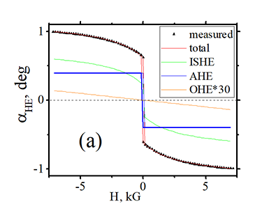
| Experiment: Measurement of Hall angle αHE in FeB nanomagnet under external magnetic field Hz. The FeB nanomagnet is fabricated on top of Ta nanowire. The Hall voltage is measured by a pair of the Hall probe. The blue balls shows the conduction electrons in the FeB, the arrows show their spin direction. In absence of magnetic field Hz. only a few spins are aligned perpendicularly to plane. These conduction electrons are called spin-polarized. Spins of other (spin-unpolarized electrons) are equally distributed in all directions. When magnetic field Hz is applied, the spins of the spin- unpolarized electrons are aligned along Hz. The larger Hz is, the more spins are aligned. As a result, the number of spin-polarized electrons becomes larger. The Hall voltage (its ISHE contribution) is linearly proportional to the number of spin-polarized electrons or the spin polarization. Therefore, the Hall voltage (and αHE) increases when magnetic field increases. |
| Measurement: The spin polarization is evaluated from a non-linear increase of αHE in external magnetic field. The measured hysteresis loop of can be divided into 3 contributions: AHE (~ constant), OHE (~H) and ISHE (~non-linear vs H). Since the dependence of the spin polarization on the magnetic field is known, the polarization s evaluated from fitting of non-linear part. |
| click on image to enlarge it |
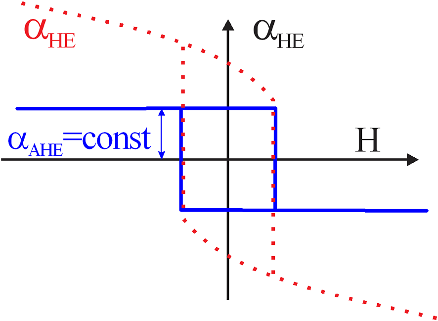
 Anomalous Hall effect (AHE)
AHE is linearly proportional to the total spin of localized electrons M.
(Dependence on external magnetic field) ![]() ~ constant
~ constant
The localized magnetic moments are firmly fixed in a ferromagnetic nanomagnet. They can only be switched between its two stable direction perpendicularly to film.
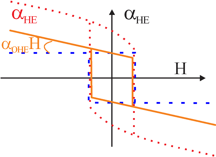
Ordinary Hall effect (OHE)OHE is linearly proportional to the magnetic field
(Dependence on external magnetic field) ![]() linear (~*H)
linear (~*H)
It is induced by the Lorentz force and therefore it is linearly proportional to external magnetic field
Inverse Spin Hall effect (ISHE)AISHE is proportional to the total spin of conduction electrons m.
(Dependence on external magnetic field) ![]() non-linear, the same as spin polarization
non-linear, the same as spin polarization
The conduction electrons are two groups: spin- polarized and spin- unpolarized electrons. In a magnetic field along spin of spin-polarized electrons, the spins of spin- unpolarized electrons are aligned along the magnetic field. As a results, the number of spin- polarized electrons becomes larger, the total magnetic moment of conduction electrons increases and the ISHE contribution increases.
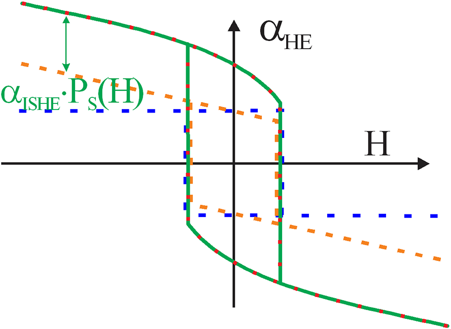
Total Hall angle αHE of nanomagnet vs. external perpendicular magnetic field H:
![]()
where αOHE is angle of the OHE contribution, which is linear vs. H ; αAHE is angle of the AHE contribution, which is independent of H ; αISHE is angle of the ISHE contribution, which is a non-linear of H ; PS (H) is the spin polarization of conduction electrons, which non-linearly increases with H.
Hysteresis loop for each contribution to Hall effect |
||||||||||||
| Red dot line shows the measured loop of Hall angle αHE | ||||||||||||
|
||||||||||||
|
||||||||||||
|---|---|---|---|---|---|---|---|---|---|---|---|---|
|
||||||||||||
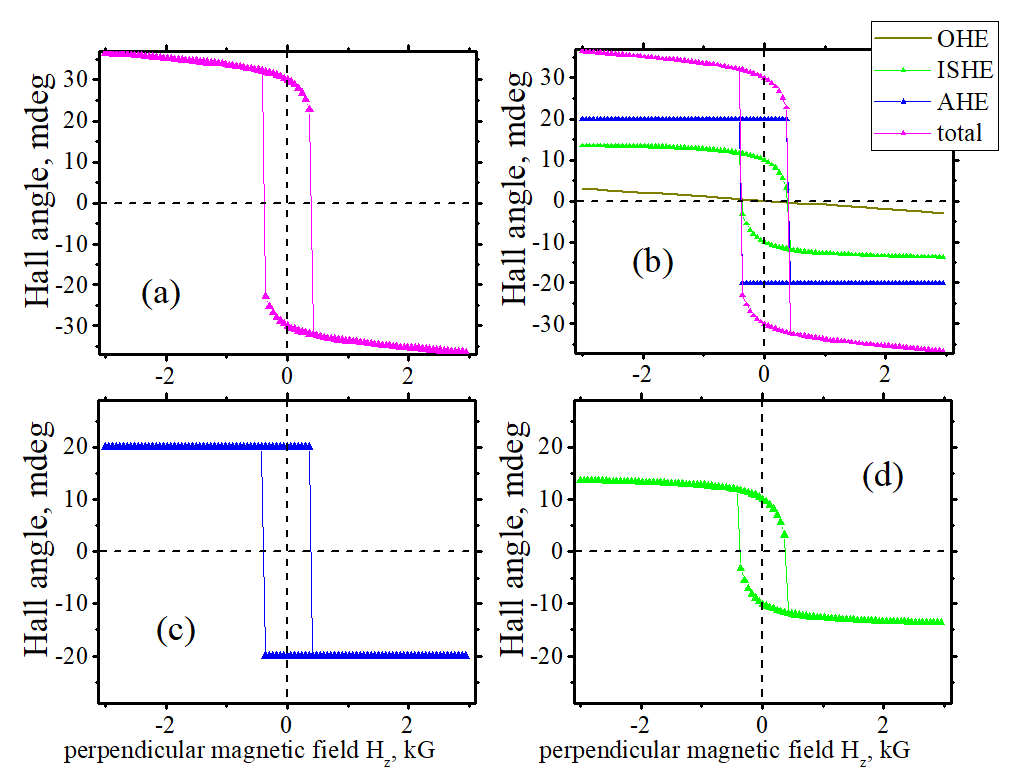
| Hall angle vs perpendicular magnetic field H. (a) Experimental data as a sum of three contributions: triangles is the total measured angle αHE(H), red line is the sum of contributions, blue/green/orange lines are individual AHE/ISHE/OHE contributions, respectively. (b) Schematic plot showing the shape of hysteresis loop for different contributions. Solid red line is the measured (total) angle. Dashed blue horizontal line is hypothetical loop in absence of OHE and ISHE. Slanted dashed orange line is loop in absence of only ISHE. Dotted green line is the loop in the hypothetical case when all conduction electrons are spin polarized sp = 100% | ||||||||||||
| Sample :Volt54B ud16 200nm 200 nm (more sample details are here) | ||||||||||||
| sp0=81.7% ; Hpump=0.834 kG ; Ta (2.5 nm):FeB(1 nm):MgO; sample: | ||||||||||||
| Click on image to enlarge it. |

Fitting of measured Hall angle |
||||||||||
|
||||||||||
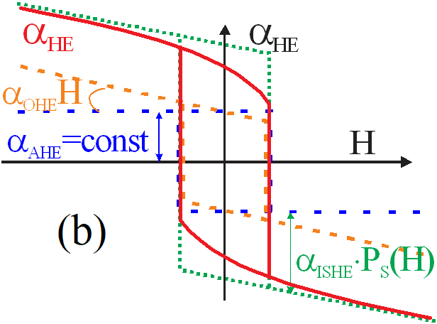
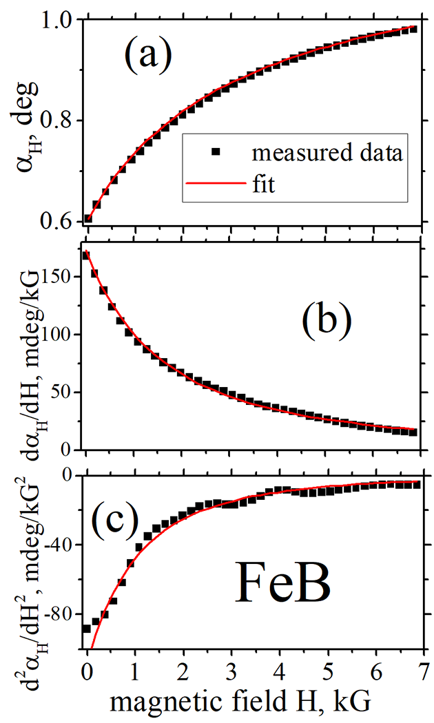
| Fig. 5. Hall rotation angle αH as a function of applied magnetic field H ; 1st and 2nd derivatives of αH Black triangles show the measured data. The red line shows the fitting by Eq.(5) | ||||||||||
| Click on image to enlarge it. |
(fact 1) ![]() The Hall angle αHall non-linearly increases under an external perpendicular magnetic field H for all measured FeB and FeCoB. As 2020.05, more than 100 nanomagnets have been measured (See here)
The Hall angle αHall non-linearly increases under an external perpendicular magnetic field H for all measured FeB and FeCoB. As 2020.05, more than 100 nanomagnets have been measured (See here)
(fact 2) ![]() All measured dependencies of αHall vs. H are perfectly fitted by Eq.(5) (a sum of OHE, AHE and ISHE contributions)
All measured dependencies of αHall vs. H are perfectly fitted by Eq.(5) (a sum of OHE, AHE and ISHE contributions)
(fact 3) ![]() The perfect fitting can be only achieved only for a small-size nanomagnet with the perpendicular magnetic anisotropy (PMA), in which the magnetization is firmly fixed perpendicularly to the surface and does not change under the magnetic field H.
The perfect fitting can be only achieved only for a small-size nanomagnet with the perpendicular magnetic anisotropy (PMA), in which the magnetization is firmly fixed perpendicularly to the surface and does not change under the magnetic field H.
(fact 4) ![]() The fitting is impossible for a large nanomagnets, in which static magnetic domains exist and the magnetization is smoothly changing under H due to movement of domain walls. (See below for details)
The fitting is impossible for a large nanomagnets, in which static magnetic domains exist and the magnetization is smoothly changing under H due to movement of domain walls. (See below for details)
(fact 5) ![]() The fitting is impossible for a continuos film, in which static magnetic domains exist and the magnetization is smoothly changing under H due to movement of domain walls.
The fitting is impossible for a continuos film, in which static magnetic domains exist and the magnetization is smoothly changing under H due to movement of domain walls.
(fact 6) ![]() The fitting is impossible for a in an antiferromagnet or a compensated ferromagnet, in which the magnetization is changing due a re- alignment of opposite spins of different magnetic super lattices.
The fitting is impossible for a in an antiferromagnet or a compensated ferromagnet, in which the magnetization is changing due a re- alignment of opposite spins of different magnetic super lattices.
(fact 7) ![]() The Hall angle in a ferromagnet always has an ISHE contribution, which makes dependence of αHall vs. H to be non-linear.
The Hall angle in a ferromagnet always has an ISHE contribution, which makes dependence of αHall vs. H to be non-linear.
(fact 8) ![]() The equilibrium spin polarization PS in FeB and FeCoB is neither zero (PS (H =0) ≠ 0) nor one (PS (H =0) ≠ 1). Otherwise, PS (H ) would linear.
The equilibrium spin polarization PS in FeB and FeCoB is neither zero (PS (H =0) ≠ 0) nor one (PS (H =0) ≠ 1). Otherwise, PS (H ) would linear.
(fact 9) ![]() The measured dependence αHall vs. H is different for different materials, different samples, and different nanomagnets See (Fig.5 on the right)
The measured dependence αHall vs. H is different for different materials, different samples, and different nanomagnets See (Fig.5 on the right)
(fact 10) ![]() The AHE contribution αAHE is slightly different for similar nanomagnets fabricated on same wafer. The ISHE contribution αISHE is sometimes different but sometimes the same for similar nanomagnets fabricated on same wafer. See below for details
The AHE contribution αAHE is slightly different for similar nanomagnets fabricated on same wafer. The ISHE contribution αISHE is sometimes different but sometimes the same for similar nanomagnets fabricated on same wafer. See below for details
Experimental setup to measure ISHE and spin polarization |
 |
| FeB nanomagnet connected to the Hall probe |
(Example structure) FeB(1nm) nanomagnet fabricated on top of Ta (3 nm) non-magnetic nanowire. Nanomagnet size is 200 nm x 20 0nm. The Hall voltage was measured by a pair of Hall probe aligned to the nanomagnet position. An external magnetic field H (red arrow) applied along the magnetization direction and perpendicularly to nanomagnet surface. |
|
| Click on image to enlarge it. |
Methods to check the absence of magnetic domains ![]()
![]()
![]()
(method 1): Smooth 1st and 2nd derivatives of vs H without any sparks or sharp steps. (See below for details)
(method 2) Similarities of 1st and 2nd derivatives for different samples (See below for details)

Method for measurement of ISHE and spin polarization |
 |
| The blue balls shows the conduction electrons in the FeB, the arrows show their spin direction. In absence of magnetic field Hz, only a few spins are aligned perpendicularly to plane. These conduction electrons are called spin-polarized. Spins of other (spin-unpolarized electrons) are equally distributed in all directions. When magnetic field Hz is applied, the spins of the spin- unpolarized electrons are aligned along Hz. The larger Hz is, the more spins are aligned. As a result, the number of spin-polarized electrons becomes larger. The Hall voltage (its ISHE contribution) is linearly proportional to the number of spin-polarized electrons or the spin polarization. Therefore, the Hall voltage (and αHE) increases when magnetic field increases. |
|
| Click on image to enlarge it. |
The spin polarization PS of the electron gas is defined as a ratio of the number of spin-polarized electrons to the total number of the spin-polarized and spin-unpolarized electrons:

where nTIA and nTIS are the numbers of spin-polarized and spin-unpolarized electrons, respectively.
In an external perpendicular magnetic field H the spin polarization increases as
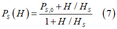
where PS,0 is the equilibrium spin polarization in absence of magnetic field (H=0); HS is the scaling magnetic field;
From Eq.7, the dependence of the Hall angle αHall on the external perpendicular magnetic field H is described by the following non-linear function
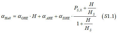
in which αOHE, αAHE, αISHE, PS,0 and HS are all independent of H.
Eq.7 was calculated from a requirement of balancing of conversion rate of spin-polarized to spin- unpolarized electrons and backward rate of of spin-unpolarized to spin- polarized electrons. See this pdf file, or below or full details here
The scaling magnetic fields HS can be calculated as (See this pdf file):
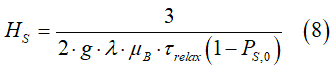
where g is the g-factor, λ is a phenomenological damping parameter of LL equation, and μB is the Bohr magneton , τrelax is the spin relaxation time
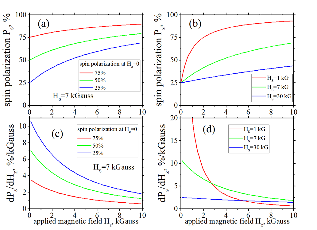
(note about HS)  The non-linearity is the key distinguish feature of the ISHE component and therefore the spin polarization is evaluated from measured non-linearity of the Hall angle. A parameter, which defines the non-linearity, is the scaling magnetic field HS. When HS becomes larger, the ISHE contribution becomes close to linear and it is difficult to distinguish it from the linear OHE contribution. For the case HS ≥ 30kG the ISHE becomes nearly- linearly (Fig. 4(b,d)) and this method stops working.
HS increases ![]() when
when
(1) spin relaxation becomes faster and the the spin relaxation decreases;
(2) spin- polarization becomes close to 100% (PS,0 ~1);
(3) spin damping becomes weaker and the damping parameter λ decreases
(bad sample)  In a sample with a larger number of defects and imperfections, the spin relaxation is larger and therefore HS is larger
Ambiguity of fitting |
 |
| Fig.5 Ambiguity of the data fitting. Experimental data (black triangle) can be perfectly fitted by two different fittings having different parameters. Parameters of 1st fitting (solid lines): PS,0= 40%, αISHE = 886 mdeg αAHE= 268 mdeg. Parameters of 2nd fitting (dash lines):PS,0=10%, αISHE = 590 mdeg αAHE= 563 mdeg. The parameters HS =3.13 kG and αOHE=0.2 mdeg/kG are the same for both fittings and therefore are evaluated unambiguously. Both fittings give the identical total Hall angle αHE and its 1st derivation |
| sample: Volt54B ud16 200nm 200 nm (more sample details are here) |
| click on image to enlarge it |
The dependence of Hall angle αHall on an external perpendicular magnetic field H in nanomagnet with PMA is described as
where αOHE is the angle of the OHE contribution, αAHE is the angle of the AHE contribution and αISHE is the angle of the ISHE contribution, PS,0 is spin polarization at H=0 and HS is the scaling magnetic field.
The ambiguity is originated from the fact that the functional dependence (S1.1) does not change when the set of three initial fitting parameters ![]() changes to a new set
changes to a new set![]() , which is related to the initial set as
, which is related to the initial set as


![]()
![]() See
See ![]() ambiguility.pdf for details.
ambiguility.pdf for details.
Figure 5 shows the measured Hall angle αHall vs. external perpendicular magnetic field H and its 1st derivative . Two perfect fittings by Eq.S1.1 are shown by the solid and dashed lines. The solid lines show the case of a higher spin polarization, a higher ISHE contribution and a smaller AHE contribution. The dashed lines show the case of a smaller spin polarization, a smaller ISHE contribution and a higher AHE contribution. There is no AHE contribution for ∂αHall/∂H (Fig. S2(b)) and there is no ambiguity for ∂αISHE/∂H.
It should be noted that the total Hall angle αHall and its derivatives are absolutely the same for both fittings (solid and dashed lines). The difference of between solid and dashed lines is a different representation of one identical function (Eq.S1.1) by different sets of parameters ![]() . There is no ambiguity for a fitting of experimental data by the function of Eq.S1.1 and there is only one function of Eq.S.11, which gives the best fit for each experimental data. However, this one function can represented by different sets of
. There is no ambiguity for a fitting of experimental data by the function of Eq.S1.1 and there is only one function of Eq.S.11, which gives the best fit for each experimental data. However, this one function can represented by different sets of ![]() .
.
The parameter HS is obtained from fitting unambiguously. The 1/HS describes the effectiveness of spin alignment along magnetic field. From LL equation, the alignment is faster when the Gilbert constant is larger. Also, the effectiveness is larger when the spin relaxation is smaller. The 1st and 2nd derivatives are larger when HS is smaller.
(Example 1) ![]() FeB of Fig.5 (a-c)
FeB of Fig.5 (a-c)
(fitting set 1)![]() HS=3.13 kG; PS,0=0.4 ;αAHE = 268 mdeg; αISHE = 886 mdeg; αOHE = 0.2 mdeg/kG;
HS=3.13 kG; PS,0=0.4 ;αAHE = 268 mdeg; αISHE = 886 mdeg; αOHE = 0.2 mdeg/kG;
(fitting set 2)![]() HS=3.13 kG;PS,0=0.3 ;αAHE = 395 mdeg; αISHE = 759 mdeg; αOHE = 0.2 mdeg/kG;
HS=3.13 kG;PS,0=0.3 ;αAHE = 395 mdeg; αISHE = 759 mdeg; αOHE = 0.2 mdeg/kG;
(fitting set 3)![]() HS=3.13 kG;PS,0=0.2 ;αAHE = 490 mdeg; αISHE = 664 mdeg; αOHE = 0.2 mdeg/kG;
HS=3.13 kG;PS,0=0.2 ;αAHE = 490 mdeg; αISHE = 664 mdeg; αOHE = 0.2 mdeg/kG;
(fitting set 4)![]() HS=3.13 kG;PS,0=0.1 ;αAHE = 563 mdeg; αISHE = 590 mdeg; αOHE = 0.2 mdeg/kG;
HS=3.13 kG;PS,0=0.1 ;αAHE = 563 mdeg; αISHE = 590 mdeg; αOHE = 0.2 mdeg/kG;
(Example 2) ![]() FeCoB of Fig.5 (e-h)
FeCoB of Fig.5 (e-h)
(fitting set 1)![]() HS=6.18 kG;PS,0=0.5 ;αAHE = 657 mdeg; αISHE = 783 mdeg; αOHE = 0.2 mdeg/kG;
HS=6.18 kG;PS,0=0.5 ;αAHE = 657 mdeg; αISHE = 783 mdeg; αOHE = 0.2 mdeg/kG;
(fitting set 2)![]() HS=6.18 kG;PS,0=0.4 ;αAHE = 788 mdeg; αISHE = 653 mdeg; αOHE = 0.2 mdeg/kG;
HS=6.18 kG;PS,0=0.4 ;αAHE = 788 mdeg; αISHE = 653 mdeg; αOHE = 0.2 mdeg/kG;
(fitting set 3)![]() HS=6.18 kG; PS,0=0.3 ;αAHE = 851 mdeg; αISHE = 560 mdeg; αOHE = 0.2 mdeg/kG;
HS=6.18 kG; PS,0=0.3 ;αAHE = 851 mdeg; αISHE = 560 mdeg; αOHE = 0.2 mdeg/kG;
(fitting set 4)![]() HS=6.18 kG;PS,0=0.2 ;αAHE = 951 mdeg; αISHE = 490 mdeg; αOHE = 0.2 mdeg/kG;
HS=6.18 kG;PS,0=0.2 ;αAHE = 951 mdeg; αISHE = 490 mdeg; αOHE = 0.2 mdeg/kG;
 Measurement procedure
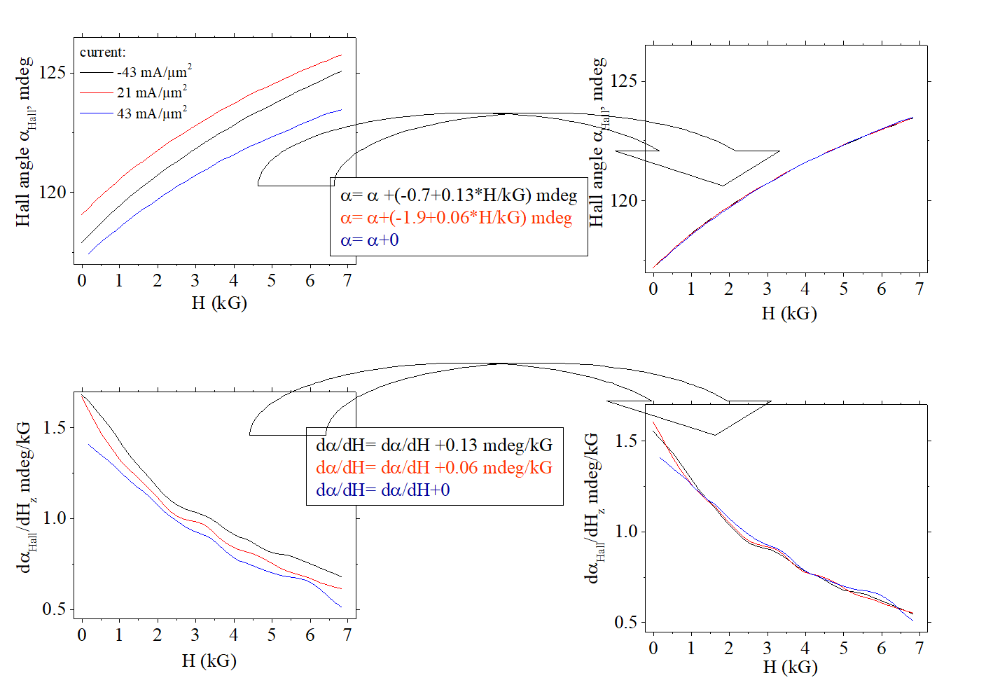 |
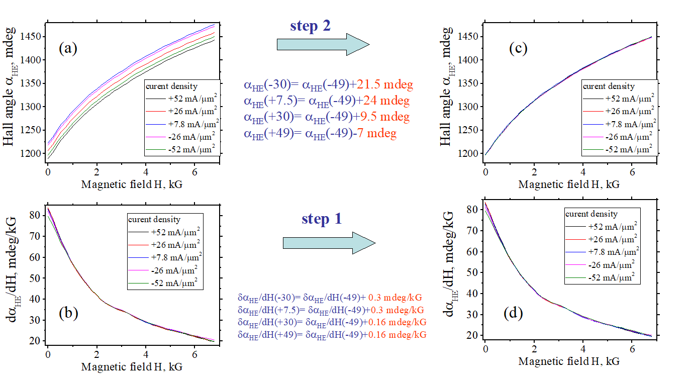
| (left side: Measured data) : Both αHall and dαHall /dHz depend on the current |
| (right side: data fitted to each other) : (step 1) (right- bottom graph): fitting of 1st derivative dαHall /dH measured at different currents into one single line (step 2) (right- top graph):. Fitting of measured αHall at different currents into one single line. After two steps all lines fit perfectly in one single line.. |
| Note: 2nd derivative behaves similar to 1st derivative |
|
| When current j is change from 43 to 23 mA/ μm2, AHE change is ΔαAHE =-1.9 mdeg and change of derivative ISHE Δ(dαISHE/dH)= 0.06 mdeg/kG |
| When current j is change from +43 to -43 mA/ μm2, AHE change is ΔαAHE = -0.7 mdeg and change of derivative ISHE Δ(dαISHE/dH)= 0.13 mdeg/kG |
| Sample: Volt57B L20 |
| Click on image to enlarge it |
Despite of existence of the ambiguity, an important information about spin polarization and its properties can be evaluated.
(point 1) ![]() The scaling field HS is evaluated unambiguously.
The scaling field HS is evaluated unambiguously.
(point 2) ![]()
![]() Even though the absolute values of ISHE and AHE contributions cannot be evaluated unambiguously, their small changes can be evaluated (e.g. when a current or gate voltage or temperature is changed)
Even though the absolute values of ISHE and AHE contributions cannot be evaluated unambiguously, their small changes can be evaluated (e.g. when a current or gate voltage or temperature is changed)
Evaluation of small changes of αAHE and αISHE. Example of Fig.23
At left side of Fig.23, the measured Hall angle αHall and its first derivative are shown for a different current density. Both the 0 and 1st derivatives are different for a different current density.
(fitting, step 1)![]() Finding change of the ISHE contribution
Finding change of the ISHE contribution
Since AHE contribution is a constant vs H, it does not contribute to the 1st derivative, the change of dαHall/dH is due a change of only the ISHE contribution. Also, all curves are clearly parallel to each other. Therefore, there is only a constant offset between them. The offset can be fitting curves to each other. In the case of Fig 23 (button raw) all curves are coincide when
dαHall/dH (black line)= dαHall/dH (blue line) +0.13 mdeg/kG
dαHall/dH (red line)= dαHall/dH (blue line) +0.06 mdeg/kG
(fitting, step 2)![]() Finding change of the AHE contribution
Finding change of the AHE contribution
When the dependence αHall vs H is corrected for the ISHE contribution, all curves of αHall (upper raw) become parallel to each other. Therefore, there is only a constant offset between them. The offset can be fitting curves to each other. In the case of Fig 23 (upper raw) all curves are coincide when
αHall(black line)=αHall(blue line) +(-0.7 mdeg +0.13 mdeg/kG *H)
αHall(red line)=αHall(blue line) +(-1.9 mdeg +0.13 mdeg/kG *H)
(result of fitting)
The change of the ISHE contribution
dαISHE/dH (-43 mA/μm2)- dαISHE/dH (43 mA/μm2) =0.13 mdeg/kG
dαISHE/dH (21 mA/μm2)= dαISHE/dH (43 mA/μm2) =0.06 mdeg/kG
The change of the AHE contribution
αAHE(-43 mA/μm2)-αAHE(43 mA/μm2) =-0.7 mdeg
αAHE (21 mA/μm2)=αAHE(43 mA/μm2) =-1.9 mdeg
(note about AHE)![]() There is almost always a detectable change of the AHE contribution when (1) current is changed or (2) gate voltage changed or (3) between different nanomagnet of one sample (4) between different samples.
There is almost always a detectable change of the AHE contribution when (1) current is changed or (2) gate voltage changed or (3) between different nanomagnet of one sample (4) between different samples.
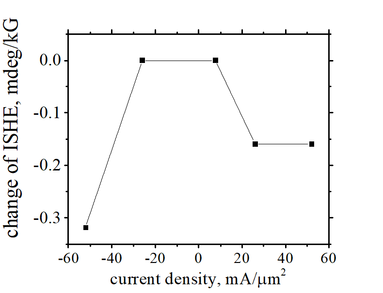
(note about ISHE)![]() For some cases the ISHE change is detectable (See Fig.23), but for some cases the ISHE change is not detectable (even when the AHE change is clearly detectable). See Fig.7 and Fig.8
For some cases the ISHE change is detectable (See Fig.23), but for some cases the ISHE change is not detectable (even when the AHE change is clearly detectable). See Fig.7 and Fig.8
The effect of Spin-Orbit torque (SOT effect) describes the fact that magnetic properties of ferromagnetic nanowire may depend on the magnitude and polarity of an electrical current flowing through the nanowire. For example, under a sufficiently large current the magnetization of the nanowire may be reversed. The direction of the magnetization reversal depends on the polarity of the current. The effect may be used as a recording mechanism for 3-terminal MRAM. The origin of the SOT effect is the spin Hall effect, which describes the fact that an electrical current may create a spin accumulation.
A. The polarity of the spin polarization generated by the Spin Hall effect are different at opposite sides of nanomagnet (see here). In the case of a symmetrical nanomagnet, the generated spin polarization is the same at opposite sides of the nanomagnet, the total generated spin polarization is zero and there is no SOT effect. Our studied samples are asymmetric. The ferromagnetic metal is contacting the MgO at one side and the Ta at another side. As a result, the total spin polarization generated by the Spin Hall effect is non-zero. However, in this case the contributions from each interface are nearly equal. It can explain the observed substantial change of the slope for different nanomagnets on the same wafer and the different slope polarities for the FeB and FeCoB samples. The enlargement of structure asymmetry and optimizing interfaces may increase the current- induced change of sp.
| Dependence of AHE and ISHE on current (temperature) and current polarity (SOT effect) | ||||||||||||||||||||||||||||||||
|---|---|---|---|---|---|---|---|---|---|---|---|---|---|---|---|---|---|---|---|---|---|---|---|---|---|---|---|---|---|---|---|---|
fitting procedure: (step 1) all line of 1st derivative are fitted into one line by adding a fitting constant. The obtained fitting constant describes the voltage- dependence of ISHE (step2) after correction of step 1, all line of 1st derivative are fitted into one line by adding a fitting constant. The obtained fitting constant describes the voltage- dependence of AHE |
||||||||||||||||||||||||||||||||
|
||||||||||||||||||||||||||||||||
| click on image to enlarge it |
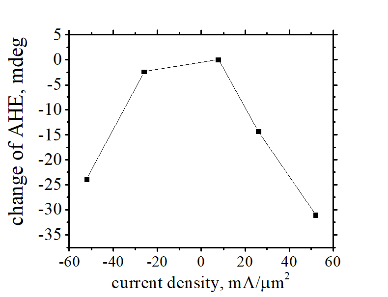
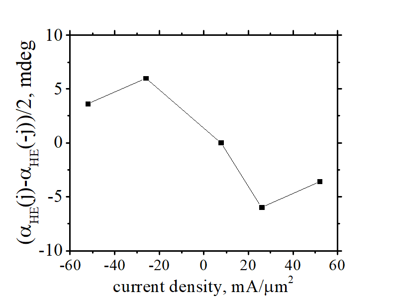
Dependence of AHE on current polarity. SOT effect |
||||||
|---|---|---|---|---|---|---|
| The data shows the difference of the Hall angle between two opposite currents | ||||||
|
||||||
| Polarity change of AHE decreases as current increases from negative to positive. There is a saturation at about 40 mA/μm2. With a little exception, such behavior is seen for the most of the samples. | ||||||
| click on image to enlarge it |
Voltage- Controlled Magnetic Anisotropy (VCMA) effect |
|---|
| Dependence of magnetic properties on gate voltage |
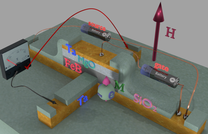
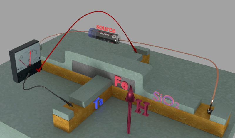
| The Hall voltage in FeB nanomagnet (shown in grey) increases are changed when a gate voltage is applied at a metal- isolator interface at the top of the nanomagnet. The source battery provides the bias current through the metallic nanowire and the nanomagnet. The voltmeter measured the Hall voltage, which is created perpendicularly to the bias current. The gate voltage is applied between the top of nanomagnet and the nanowire. Because of thick (~ 10 nm) gate isolator (MgO), the gate voltage does not induce any electrical current. The effect, which describes the dependence of the magnetic properties on the gate voltage, is called the Voltage- Controlled Magnetic Anisotropy (VCMA). See details here. |
| click on image to enlarge it |
The VCMA effect describes the fact that in a capacitor, in which one of the electrodes is made of a thin ferromagnetic metal, the magnetic properties of the ferromagnetic metal are changed, when a voltage is applied to the capacitor. For example, under an applied voltage the magnetization direction of the ferromagnetic metal may be changed or even reversed. This magnetization-switching mechanism can be used as a data recording method for low-power magnetic random access memory and all metal transistor. Until now the physical origin of the VCMA effect has not been clarified. However, several possible physical mechanisms have been discussed. (See here for more details)
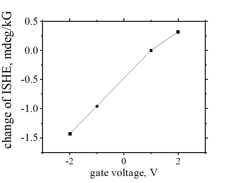
A. I guess there are several contributions to the bias-dependence of TMR. The voltage dependence may have some contribution. However, it should be a contribution, which is polarity dependent. The voltage-control change of the spin polarization always changes its sign, when the voltage polarity is reversed. I have checked many samples already. The spin polarization always linearly increases under a negative gate voltage and it always linearly decrease under a positive gate voltage.
| Dependence of AHE and ISHE on gate voltage (VCMA effect) | ||||||||||||||||||||||||||||||||
|---|---|---|---|---|---|---|---|---|---|---|---|---|---|---|---|---|---|---|---|---|---|---|---|---|---|---|---|---|---|---|---|---|
fitting procedure: (step 1) all line of 1st derivative are fitted into one line by adding a fitting constant. The obtained fitting constant describes the voltage- dependence of ISHE (step2) after correction of step 1, all line of 1st derivative are fitted into one line by adding a fitting constant. The obtained fitting constant describes the voltage- dependence of AHE |
||||||||||||||||||||||||||||||||
|
||||||||||||||||||||||||||||||||
| click on image to enlarge it |
Methods to measure of spin polarization of conduction electrons |
|||
|
|||
|
|||
|
|||
Spin polarization sp of conduction electrons is evaluated from measured dependence of αHall or θFaraday or θKerr or μtotal on the external magnetic field H. |
|||
|---|---|---|---|
| All these methods are direct methods to measure the spin polarization, because they measure the magnetization of the conduction electrons and therefore the number of the spin- polarized conduction electrons. |
It requires to measure a material property, which depends on the spin polarization (i.e. Hall angle, a MO constant, sample magnetization, tunnel resistance etc). In order to evaluate the spin polarization, the spin polarization is changed in controllable way and the dependence of the material property on the change of the spin polarization is measured. From a fitting of measured data to the known dependence of the material property on the spin polarization , the absolute value of the spin polarization is evaluated.
In the below-described method, the dependence of the Hall angle on an applied magnetic field is measured.
Similarly, the measurements of the dependence of the magneto-optical (MO) constants or the tunnel resistance or the magnetization measured by a magnetometer on modulated spin polarization are also the effective methods to measure the spin polarization of the conduction electrons.
![]() The spin polarization can be changed by applying an external magnetic field, by applying the elastic stress, by illuminating the sample by circular- polarized light, by injecting spin-polarized electrons from another metal.
The spin polarization can be changed by applying an external magnetic field, by applying the elastic stress, by illuminating the sample by circular- polarized light, by injecting spin-polarized electrons from another metal.
In the below- described method, the spin polarization is modulated by applying an external magnetic field Hext along the spin direction of the spin polarized electrons.
The spin polarization increases when a magnetic field is applied along spin direction of the spin-polarized electrons.(The reason why it increases): The spins of spin unpolarized electrons are aligned along the magnetic field. As a result, the number of spin- polarized electrons becomes larger. The process of spin alignment is described by the Gilbert damping parameter in the Landau- Lifshitz equations (See here)
 When the spin polarization sp of the conduction electrons changes, the amount of the spin-polarized conduction electrons changes and therefore the total magnetic moment of the conduction electrons changes as well. Nearly-all magnetic properties depends on the the total magnetic moment of the conduction electrons. Specifically the Hall angle, magneto-optical constant, the total magnetic moment and all magneto-transport properties are changed when the spin polarization is changed.
Main condition is that under applying of an external magnetic field only the spin polarization of the conduction electrons changes, but all other parameters remain unchanged. It means that
(condition 1) The magnetic field is applied along magnetization and the spin direction of the spin polarized electrons. The magnetization direction remains along magnetic field during the whole measurement.
(condition 2) There are no any magnetic domains. Over whole sample, the magnetization is directed along the external magnetic field for any used values of the magnetic field.
(condition 3) The temperature, bias current etc. remain unchanged during the whole measurement
In any measurement of the spin polarization, the change of a material parameter is traced under a change of spin polarization of conduction electrons. The simplest way to change the spin polarization of the conduction electrons is to apply an external magnetic field. However, it is possible to evaluate the spin polarization only if one parameter, the spin polarization changes under the external magnetic field and all other parameters remains unchanged. E.g. in the case when there is a movement of magnetic domain under an increasing magnetic field, the evaluation of the spin polarization is impossible.
A. All below-described measurement methods are based on a measurement of the magnetization of the conduction electrons. The magnetization of the conduction electrons is the sum of the magnetization of each spin-polarized electrons and therefore it is linearly proportional to the number of the spin- polarized conduction electrons.
Additional merit of a direct measurement of sp is that the magnetization of the conduction electrons has distinguished symmetry properties, which can be verified and a possible systematic error can be avoided.
![]() A general form of dependency of material parameters on different magnetic properties can be found from symmetry rules. The most of important magnetic properties can be found from the TCP symmetry. In the following more simplified symmetry rules are used
A general form of dependency of material parameters on different magnetic properties can be found from symmetry rules. The most of important magnetic properties can be found from the TCP symmetry. In the following more simplified symmetry rules are used
A measurement of the spin polarization required that the sample is always fully-saturated without any magnetic domains. It means that after the external magnetic field His reversed, the magnetization, the spins of d- electrons and spin of conduction electrons are fully reversing following H.
From the symmetry, any material parameter, which reverses its sign, when the external magnetic field is reversed can be calculated as
![]()
where a,b,c are constants, which sign is not reversed under reversal of H, Scond is the total spin of the conduction electrons, and Sd is the total spin of the localized d-electrons
Magnetic parameters, which reversed with reversal of external magnetic field: (1) magnetization M or the total magnetic moment of localized d-electrons Md, (2) the total magnetic moment of spin polarized electrons Mcond ; (3) the Hall voltage and the Hall angle αHall; (4) magneto-optical constants: Faraday rotation angle θFaraday , the Kerr rotation angle, constants of magnetic circular dichroism (MCD).
method 1: Hall measurement |
||||||
|
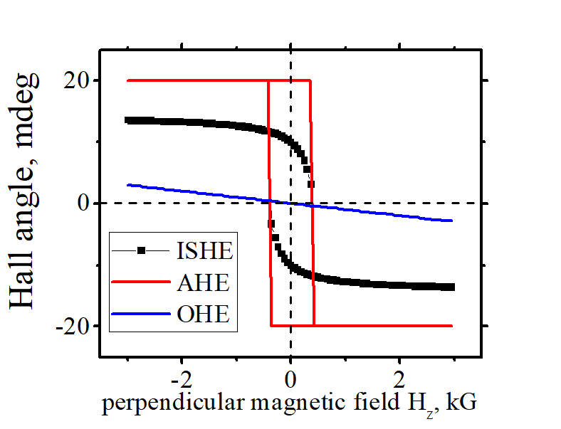
||||||
| Hall angle αHall has 3 contributions: (1st linear contribution (blue line)) Ordinary Hall effect (OHE); (2d constant contribution (red line)) Anomalous Hall effect (AHE); (3d non- linear contribution (black line)) Inverse Spin Hall effect (ISHE); | ||||||
Since ISHE contribution depends of the spin polarization sp of conduction electrons, fitting of measured αHall gives spin polarization sp of conduction electrons. |
||||||
|---|---|---|---|---|---|---|
| Click on image to enlarge it. |
 Measurement of spin polarization.
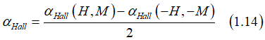
 The Hall angle αHall is asymmetrical with respect to H reversal. Therefore, it defines as a difference of αHall measured at opposite H:
![]()
αHall can be linearly proportional to material parameters of the same symmetry![]()
where Md is the total magnetic moment of localized d-electrons and Mcond is the total magnetic moment of conduction electrons. The total moment of all spin-unpolarized electrons is zero. Since all spins spin-polarized electrons are directed in one direction, Mcond =μcond ·nTIA , where nTIA is the number of spin-polarized conduction electrons, μcond is the magnetic moment of one conduction electron.
Therefore, Eq(3.2) is simplified as
![]()
nd is the number of spin-active localized d-electrons and μd is the magnetic moment of one localized d- electron.
By definition of the spin polarization sp (See here) is percentage of spin-polarized electron among conduction electrons:
where ncond is the total number of spin-polarized and unpolarized electrons.
The magnetization M of a ferromagnetic metal is defined as
Substitution of Eqs. (3.0) and (3.0a) gives
![]()
or ![]()
where βISHE is redefined as βISHE =βISHE· μcond ·ncond
The ![]() 1st term βOHE·H describes proportionality of αHall to external magnetic field. This effect is called the ordinary Hall effect.
1st term βOHE·H describes proportionality of αHall to external magnetic field. This effect is called the ordinary Hall effect.
The ![]() 2nd term βAHE·M describes proportionality of αHall to magnetization of the ferromagnetic metal. This effect is called the Anomalous Hall effect.
2nd term βAHE·M describes proportionality of αHall to magnetization of the ferromagnetic metal. This effect is called the Anomalous Hall effect.
The ![]() 3d term βISHE·sp describes proportionality of αHall to the spin polarization of the conduction electrons. This effect is called the Inverse Spin Hall effect.
3d term βISHE·sp describes proportionality of αHall to the spin polarization of the conduction electrons. This effect is called the Inverse Spin Hall effect.
method 2: magneto-optical measurement |
||||||
|
||||||
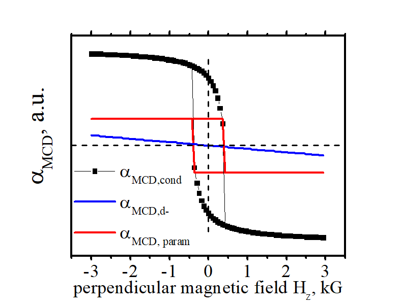
| (left) Total measured αMCD has has 3 contributions: (1st non-linear contribution, black line) contribution of spin-polarized conduction electrons αMCD,cond ;, which is proportional to the number of the conduction electrons; (2d constant contribution, red line) contribution of d-electron αMCD,d-, which is proportional to the number of the d- electrons; (3d linear contribution) paramagnetic contribution αMCD,param , which is due transition of paramagnetic electrons. | ||||||
Since αMCD,cond depends of the number of spin-polarized electrons and therefore on the spin polarization sp of conduction electrons, fitting of measured αMCD gives spin polarization sp of conduction electrons. |
||||||
|---|---|---|---|---|---|---|
| Click on image to enlarge it. |
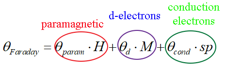
A measurement of the Faraday rotation angle θFaraday or Kerr rotation angle θKerr or difference in absorption between left- and right circular polarized light (MCD effect) can be used to evaluate the spin polarization of conduction electrons. The following explains how the spin polarization can be evaluate from a measurement the MCD absorption. Similar evaluation can be done from a measurement of Faraday rotation angle θFaraday or Kerr rotation angle θKerr.
A circular polarized photon has spin equals 1. Therefore, a spin polarized electron can be excited only, for example, by left-, but not by right circular light as it required by the Selection rules for electronic transition.
In the case when there are spin-polarized electrons, the absorption of left- and right circular polarized becomes different. This effect is called the magnetic Circular Dichroism.(See here and here and here)
The difference in absorption coefficient αMCD between left and right circular polarized light changes its sign, when spin direction of the spin polarized electron is reversed. When spins are reversed by external magnetic field H, αMCD can be measured as
![]()
Measurement of spacial distribution of spin polarization in GaAs. Optical spin injection |
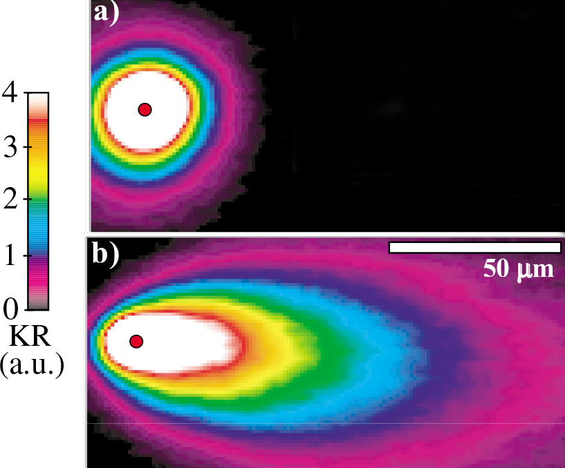 |
| Spacial distribution of Kerr rotation angle in GaAs. Red circle shows the spot, at which focused circular polarized light excites spin-polarized electrons. The Kerr rotation angle is proportional to spin polarization sp of the conduction electrons. The spin polarization decays as the photo-excited electrons diffuse from the laser spot. (a) The electrical field is not applied. The spin polarization decays symmetrically in all directions. (b) Electrical field is applied ("+" at the right and "-" at the left). As the electrons are drifted along the electrical field, the spin polarization is drifted as well. |
|
|---|
S. A. Crooker and D. L. Smith, PRL 94, 236601 (2005). Permission |
| Click on image to enlarge it. |
Each spin-polarized electrons contribute to αMCD, therefor αMCD is proportional to the number of spin-polarized electrons. Since the symmetry and size of the localized d-electrons and conduction electrons are very different, therefore the interaction efficiency of these electrons with photons is very different and these spin-polarized electrons contribute differently to αMCD. Additionally, there is a paramagnetic contribution due to the Zeeman splitting.
![]()
Eq.(3.12) can be obtained also the symmetry fact (like that αMCD
Substitution of Eqs. (3.0) and (3.0a) gives
![]()
where we redefine
method 3: measurement of magnetic moment |
||||||
|
||||||
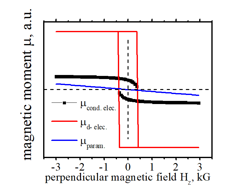
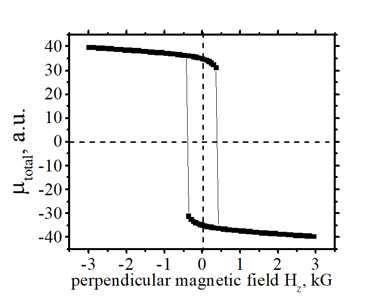
| (left) Total measured magnetic moment μtotal has has 3 contributions: (1st non- linear contribution, black line) total magnetic moment of conduction electrons μcond.elec;, which is proportional to the number of the conduction electrons; (2d constant contribution, red line) total magnetic moment of d-electrons μd-.elec, which is proportional to the number of the d- electrons; (3d linear contribution) paramagnetic moment μd-.elec, which is contribution of a substrate and paramagnetic electrons. | ||||||
Since μcond.elec depends of the number of spin-polarized electrons and therefore on the spin polarization sp of conduction electrons, fitting of measured μtotal gives spin polarization sp of conduction electrons. |
||||||
|---|---|---|---|---|---|---|
| Click on image to enlarge it. |
 Measurement of spin polarization.(Method 3): Measurement of Magnetic moment
The magnetic moment μtotal of a sample can be measured by magnetometer (SQUID or VCM)
Similarly, the magnetic moment should be reversed, when the external magnetic field is reversed
![]()
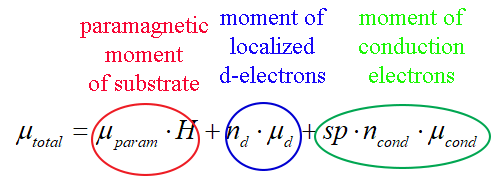
The total measured magnetic moment μtotal is the sum of magnetic moments of d-electrons, magnetic moments of the spin-polarized conduction electrons and induced magnetic moment (paramagnetic type)
![]()
Substitution of Eqs. (3.0) and (3.0a) gives
![]()
requirements of the measurement of sp:
(requirement 1): The measured material parameter should be dependent on spin polarization sp of conduction electrons (magnetization of conduction electrons).
(requirement 2): The spin polarization sp should be changed in controllable way. Therefore, the dependence of the material parameter on the spin polarization can be measured and the spin polarization sp can be found from a fitting.
change of spin polarization sp. (Method 1)![]() Applying a magnetic field along the spin direction of spin-polarized electrons.
Applying a magnetic field along the spin direction of spin-polarized electrons.
It is the most simple method and the most favorable method.
An external magnetic field aligns the spin of the spin-unpolarized electrons. As a result, the spin polarization of the conduction electrons increases (See details here)
change of spin polarization sp. (Method 2)![]() Applying a magnetic field perpendicularly to the spin direction of spin-polarized electrons. (Hanle effect)
Applying a magnetic field perpendicularly to the spin direction of spin-polarized electrons. (Hanle effect)
The perpendicular magnetic field reduces the spin polarization. Additionally, the direction of the spin polarization slightly tilts towards the magnetic field.
Ferromagnetic metal:
It is difficult to use this method for a ferromagnetic metal because (1) There is a substantial intrinsic magnetic field inside a ferromagnetic metal. The external magnetic field should be comparable with this field in order to produce any changes. (2) The magnetization and therefore the spin polarization turns towards the magnetic field.
Non-magnetic metal:
change of spin polarization sp. (Method 3)![]() Spin injection
Spin injection
The
A. All these methods are based on a measurement of complex dependencies of a material property on the spin polarization of the conduction electrons, like the tunneling resistance, spin-dependent photoluminescence, spin-dependent electroluminescence.
These methods are indirect, because the measurement material properties depends not only on sp, but on many other parameters. It is very hard to distinguish the material- property dependence on sp from similar dependencies on another material properties. E.g. additionally sp-dependence the tunneling magneto resistance depends on shape, size and symmetry of electron wavefunction in the tunnel barrier and in electrode near interface. All these these parameters may or may not be spin-dependent..
These methods are exotic, because the physics of the spin-dependent tunneling and the spin-dependent photoluminescence are complex and are not fully understood yet. It is very speculative when the spin polarization is estimated from a fitting of very-approximate and suggested dependencies of the complex properties on the spin polarization.
![]() Measurement 1: From tunneling magneto-resistance (TMR) using Julliere formula
Measurement 1: From tunneling magneto-resistance (TMR) using Julliere formula
The TMR ratio of a magnetic tunnel junction (MTJ) is proportional to the spin polarization of its electrodes. In the most simplified case, the TMR ratio
Estimated spin polarization for FeCoB: 70-90 %
merits: Simplicity of measurements
demerits: systematic error due to substantial limitations and approximations of Julliere formula (e.g. ![]() )
)
![]() Measurement 2: from Andreev reflection
Measurement 2: from Andreev reflection
The spin polarization is evaluated from the tunneling properties of a superconductor-metal contact.
Estimated spin polarization for FeCoB: 30-50 %
merits: ???
demerits: (1) limitation of only a low temperature measurement; (2) a systematic error due to simplifications and approximations for calculations of the transport through a superconductor-metal contact; (3) clear under estimation of the value of the spin polarization;
![]() Measurement 3: using spin-dependent photoluminescence, spin-dependent electroluminescence and spin LED
Measurement 3: using spin-dependent photoluminescence, spin-dependent electroluminescence and spin LED
The spin polarization is evaluated from the amount of circular-polarized light emitted from a semiconductor, in which spin-polarized current is injected
Estimated spin polarization for FeCoB: 60-95 %
merits: (1) spatial distribution of spin polarization can be checked.
demerits: (1) incorrect description of spin injection can cause a systematic error; (2) incorrect description of complex features of spin-light interaction can cause a systematic error; (see here and here);
![]() Measurement 4: from spin-injection and spin-detection experiment (non-local spin-detection)
Measurement 4: from spin-injection and spin-detection experiment (non-local spin-detection)
In the non-local spin- detection experiment, the spin-polarized electrons are injected by a pair of ferromagnetic electrodes and detected by another pair of ferromagnetic electrodes. From dependence of the spin- detection voltage of different parameters of the measurement and device structure, a very rough estimation of the injected spin polarization in the paramagnetic metal and the spin polarization of ferromagnetic electrodes can be obtained.
merits: (1) simplicity of experiment
demerits: (1) all features of the spin injection and the spin detection have not been understood yet; (2) both the spin injection and the spin detection substantially depend on the quality and chemistry of interface between non-magnetic and magnetic materials.
Increase of spin polarization vs H increase makes the loop non-linear |
Spin polarization increases in a magnetic field due to precession damping | |
|---|---|---|
 |
 |
|
| The spin polarization is evaluated from non-linear dependence of Hall angle αHall on H. The green dash line shows the imaginary case if spin polarization would not depend on magnetic field. The red dot line shows the case when spin polarization of metal is close to 100 %.Click on image to enlarge it. | Fig. 1(b)Spin precession and precession damping in a magnetic field Hext . During the precession the spin aligns itself along the direction of the magnetic field. Click on the image to enlarge it. |
![]() Merit 1: Simplicity of measurements
Merit 1: Simplicity of measurements
![]() Merit 2: ability for measurement of spin-polarization even in a nano- sized object;
Merit 2: ability for measurement of spin-polarization even in a nano- sized object;
![]() The spin polarization is evaluated from the measured dependency of the Hall angle on an applied perpendicular magnetic field
The spin polarization is evaluated from the measured dependency of the Hall angle on an applied perpendicular magnetic field
Measurement of spin polarization |
 |
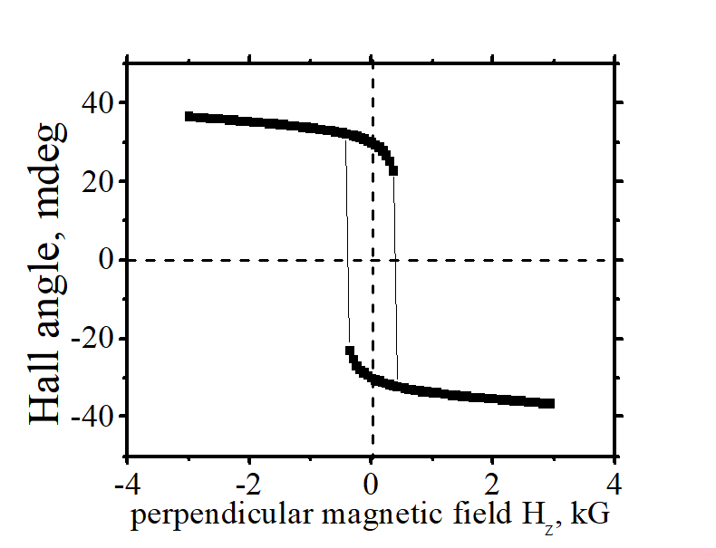
| Measured spin polarization as a function of an external magnetic field |
Volt 54B ud40 Ta(2.5)/FeB(1.1)/ MgO(6)/ nanowire width 1000 nm nanomagnet length 500 nm. Fit by Eq.(1.8) gives (region of nanomagnet):sp0=81.2% ; Hpump=0.425 kG ; |
| Click on image to enlarge it. |
Spin polarization sp in a magnetic field is calculated as
where sp0 is the spin polarization in absence of an external magnetic field, Hpump is the pumping magnetic field (a material parameter)
The measured Hall angle αHall is the sum of the Hall angle αOHE of the ordinary Hall effect, the Hall angle αAHE of the anomalous Hall effect and the Hall angle αISHE of the inverse spin Hall effect. It can be calculated as
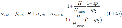
where αAHE is the Hall angle of Anomalous Hall effect, αISHE,0 is the Hall angle of the Inverse Hall effect in the absence of an external magnetic field, βOHE is the Hall coefficient of ordinary Hall effect; H⊥ is the magnetic field applied perpendicularly to the film.
Measurement of spin polarization |
|||||||||
|
|||||||||
| Hall rotation angle αHall as a function of applied magnetic field H ; 1st and 2nd derivatives of αHall normalized to its value at H=0. Black triangles show the measured data. The red line shows the fitting by Eq.(1.12) | |||||||||
| Click on image to enlarge it. |
A. The contribution of the ordinary Hall effect (OHE) depends linearly on the magnetic field . The experimentally measured dependence is non-linear and it has three contributions ![]() the linear contribution due to OHE, constant contribution due to AHE and
the linear contribution due to OHE, constant contribution due to AHE and ![]() non- linear contribution due to ISHE with respect to magnitude of external magnetic field H.
non- linear contribution due to ISHE with respect to magnitude of external magnetic field H.
A. The αISHE is linearly proportional to spin polarization (sp) of electron gas, the magnetization and the strength of the spin-orbit (SO) interaction (See details here). The strength of the SO interaction mainly depends on the ratio of the holes and electrons in a metal. Therefore, it can be assumed that it does not change in an external magnetic field. In this case the Hall angle αAHE can be calculated as
where σxx, σxy are diagonal and off-diagonal components of the conductivity tensor; a is the proportionality constant;M⊥ is out-of-plane component of magnetization
(1) major contribution: an increase of spin polarization due to increase of spin pumping
(2) minor contribution: an increase of spin polarization due to decrease of spin relaxation
(2) minor & major contribution: a change of magnetization M⊥
Measurement of spin polarization |
 |
| Fig.2. A Fe nanomagnet connected to the Hall probe |
|
| Click on image to enlarge it. |
The spin polarization of a nanomagnet was evaluated using a Hall measurement
The FeB, FeCoB and FeTbB films were grown on a Si/SiO2 substrate by sputtering. A Ta layer was used as non-magnetic adhesion layer. A nanowire of different width between 100 and 3000 nm with a Hall probe was fabricated by the argon milling. The width of the Hall probe is 50 nm. The FeB and FeCoB layers were etched out from top of the nanowire except a small region of the nanomagnet, which was aligned to the Hall probe. The nanomagnets of different lengths between 100 nm to 3000 nm were fabricated.
When it is not mentioned, the Hall angle is measured at current density of 5 mA/mm2. The aHall in the ferromagnetic metal was evaluated as

where sferro , snonMag are conductivities of ferromagnetic and non-magnetic metals; tferro , tnonMag are their thicknesses, VHall is the measured Hall voltage, I is the bias current and R,L,w are the resistance, length and width of the nanowire, correspondingly.
Each of aISHE, aAHE and aOHE reverse its sign, when M and H are reversed. In order to avoid a systematic error due to a possible misalignment of the Hall probe, the Hall angle was measured as
All conduction electrons in a ferromagnetic metal can be divided into groups of spin-polarized and spin-unpolarized electrons. The spin polarization sp of the electron gas is defined as a ratio of the number of spin-polarized electrons to the total number of the spin-polarized and spin-unpolarized electrons:
where nTIA and nTIS are the numbers of spin-polarized and spin-unpolarized electrons, respectively.
Detailed explanation is here. Explanation in short:
In fact, all conduction electrons in a ferromagnetic metal are divided into 3 groups: of spin-polarized, spin-unpolarized electrons and spin-inactive electrons. In the group of the spin-polarized electrons, the spins of all electrons are in the same direction. In the group of the spin-unpolarized electrons, the spins are distributed equally in all directions. Additionally, there are some electrons, which are "spin-inactive". A pair of these electrons with opposite spins occupies one quantum state. The occupation of quantum states by the electrons of both the spin-polarized and spin-unpolarized groups is one electron per a state. As a result, the spin of each state is 1/2 and the spin direction for each quantum state is defined. The spin direction represents the direction of the local breaking of the time-inverse symmetry for the state. When a quantum state is occupied by two conduction electrons of opposite spins, the spin of such quantum state is zero. As a result, the spin direction of this state cannot be defined and the electrons occupying this state are "spin-inactive". The electrons, which energy is substantially below the Fermi energy, mainly belong to this group. For example, nearly all of the “deep level” electrons belong to this group. In contrast, the energy of electrons of the groups of spin-polarized and spin-unpolarized electrons is distributed mainly nearly the Fermi energy. See details here.
Increase of Hall angle in external magnetic field due to increase of the spin polarization |
|||||||||
|
|||||||||
|
|||||||||
| Hall rotation angle αHall as a function of applied magnetic field H ; 1st and 2nd derivatives of αHall normalized to its value at H=0. Black triangles show the measured data. The red line shows the fitting by Eq.(1.12) | |||||||||
| Click on image to enlarge it. |
![]() Main idea:
Main idea:
![]() The spin polarization is evaluated from the measured dependency of the Hall angle on an applied perpendicular magnetic field
The spin polarization is evaluated from the measured dependency of the Hall angle on an applied perpendicular magnetic field
The spin polarization sp of the electron gas is defined as a ratio of the number of spin-polarized electrons to the total number of the spin-polarized and spin-unpolarized electrons. The amount of electrons in each group is determined by a balance between the spin pumping and the spin relaxation. The spin pumping is the conversion of electrons from groups of spin-unpolarized electrons into the group of the spin-polarized electrons. The spin relaxation is the conversion in the opposite direction.
![]() Spin-pumping rate:
Spin-pumping rate:
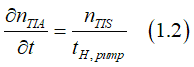
The spin pumping describes the conversion of electrons from the group of the spin-polarized electrons into the group of spin-unpolarized electrons. The conversion rate of the spin-pumping is described as
where tpump is the spin pumping time, nTIA and nTIS are the numbers of spin-polarized and spin-unpolarized electrons, respectively.
![]() Spin-relaxation rate:
Spin-relaxation rate:
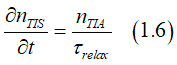
The spin damping describes the conversion of electrons from the group of the spin-polarized electrons into the group of spin-unpolarized electrons. The conversion rate of spin-relaxation can be described as
where trelax is the spin relaxation time.
![]() Spin polarization:
Spin polarization:
The spin polarization sp of electron gas can be found from the condition that in an equilibrium there is a balance between the spin pumping and the spin relaxation, which is described by the condition:

 (2) Decrease of spin relaxation rate
| Alignment of spins of conduction electrons along a magnetic field is the reason of increase of the spin polarization of the electron gas | ||||
|---|---|---|---|---|
|
||||
There are ![]() two reasons:
two reasons:
It is due to alignment of spins of spin-unpolarized electrons along a magnetic field (see Fig. 3)
![]() Spin-pumping rate induced by a magnetic field:
Spin-pumping rate induced by a magnetic field:
In a magnetic field, the spins of spin-unpolarized electrons aligns along the magnetic field due to the precession damping (See here). However, scatterings quickly re aligns spins of electrons into two groups of spin- polarized (all spins are one direction) and spin-unpolarized electrons (spins are equally distributed in all directions). (details See here) As a result, there are more spin-polarized electrons. The spin-pumping (See Eq.19 below)
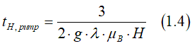
where tH,pump is the spin pumping time in a magnetic field. The spin pumping time in a magnetic field can be calculated as
![]() spin polarization of electron gas in a magnetic field
spin polarization of electron gas in a magnetic field
The spin polarization sp of electron gas can be found from the condition that in an equilibrium there is a balance between the spin pumping and the spin relaxation, which is described from Eqs (1.2),(1.5) (1.6) by the condition:
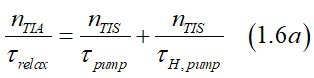
Substitution Eqs.(1.2) (1.6) Eq(1.7) into Eq.(1.1) gives the spin polarization sp of electron gas in a magnetic field (see more details here) as
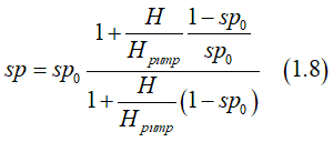
where sp0 is the spin polarization in absence of an external magnetic field (a material parameter) , which is calculated as
Hpump is the pumping magnetic field (a material parameter), which is calculated as
In described measurements it was assumed that the increase of the Hall angle in a magnetic field is only due to the increase of spin polarization, which is induced by the spin pumping induced by the magnetic field.
However,there are additional effect, which may also contribute to the increase of the spin polarization:
(1) Reduction of spin relaxation;
(2) Increase of magnetization
Absolutely. An external magnetic field reduces the spin relaxation. This reduction should be included into an evaluation of the spin polarization.
An external magnetic field reduces all mechanism of the spin relaxation:
reduction of mechanism 1 : the spin-dependent scatterings: Even spin may be rotated after a spin-dependent scattering, in a magnetic field it quickly rotates back to be along the magnetic field. Therefore, the spin- dependent scattering does not lead to the increase of the spin relaxation.
reduction of mechanism 2 : incoherent spin precession in a spatially inhomogeneous magnetic field: A large magnetic field levels out and fully compensates any possible inhomogeneities of internal magnetic field in a metal. A magnetic field reduces or even this type of the spin relaxation.
A. It does influence very much. (1). Magnetization inclination. Keeping the magnetization in the same direction is very important for these measurements. The sample geometry and the scan range of magnetic field should chosen to avoid any (even slight) magnetization inclination or domain movement. (2) Change of magnetization magnitude. In a magnetic field the spin polarization sp increases. The increase of sp may cause the increase of the magnetization as well. The amount of increase of the magnetization is difficult to measure. The correct measurement of such increase is still a challenging task.
Oscillations of measured 2nd derivative vs H |
||||||
|
||||||
| There are clear oscillations of measured 2nd derivative of αAHE vs H of an unknown origin. | ||||||
| Click on image to enlarge it. |
The physical origin of the oscillations is not yet understood.
The oscillations exists for all measured samples.
The period and amplitude of the oscillations are different from a sample to sample
nanowire with two pairs of Hall probes |
|||||||||
|
|||||||||
Volt 54B ud40 Ta(2.5)/FeB(1.1)/ MgO(6)/ nanowire width 1000 nm nanomagnet length 500 nm. Sample is soft. Hc~0 Oe, Hani~1.7 kG, |
|||||||||
| click on image to enlarge it |
Measurement of spin polarization. Comparison of different thicknesses of the same nanowire |
|||||||||
|
|||||||||
|
|||||||||
| Volt 54B ud40 Ta(2.5)/FeB(1.1)/ MgO(6)/ nanowire width 1000 nm nanomagnet length 500 nm. Sample is soft. Hc~0 Oe, Hani~1.7 kG, | |||||||||
triangles show the measured data. The solid line shows the fitting by Eq.(1.12) |
|||||||||
| Click on image to enlarge it. |
Undesirable influence of static domains |
||
|
||
Fig.6 Influence of static domain on the measurement of the Hall angle αHE. (a,d) Hysteresis loop. (b,e) absolute value of the Hall angle αHE. (c) Derivative ∂ αHE/∂H. The loop is divided into 4 parts showed by different colors. The yellow line is scan from the largest negative field until up- switching. The red line is scan from the up- switching until the largest positive field. The green line is back scan from the largest positive field until the down- switching. The blue line is scan from the down switching until the largest negative field. (a,b,c) Data of a larger 3µm x 3µm FeCoB nanomagnet. There are spark changes of the derivative in the regions of existence of static domains. (d,e,f) Data of a smaller 200nm x 200nm FeB nanomagnet. The dependencies are smooth without sparks. |
||
| sample (a,b,c) Volt 58A R41C size 3µm x 3µm (more sample details are here); sample (d,e,f) Volt54B ud16 200nm 200 nm (more sample details are here) | ||
| click on image to enlarge it |
The important requirement for our measurements is the mono domain nature of the specimen which ensures stability of the localized moment in the external magnetic field. This stability is very important to exclude any possible contribution to the Hall effect due to a realignment of localized moments. A small size of the nanomagnet ensures the absence of static magnetic domain and the stability of the localized moments.
![]()
![]()
![]() In our measurements the existence of static domains can be clearly identified. Figures 6 (a,b,c) shows measurement of the Hall angle ant its 1st derivative for a relatively- large (3µm x 3µm) FeCoB nanomagnet. At magnetic field less than 1.5 kG, there is a spark-like change of the 1st derivative indicating existence of static magnetic domains in this range of the magnetic field H. The spark- like change is due the fast realignment of localized magnetic moments during a nucleation of static domain and movement of a domain wall across the nanomagnet (See more about static magnetic domains here). Additionally, there is a dependence of the 1st derivative on the scan direction of the magnetic field. The yellow and green lines are different from the red and blue lines for |H| <1.5 kG. It is an indication of an existence of a thermally- activated mechanism, which is probably a mechanism to overcome obstacles during movement of a domain-wall across the nanomagnet.
In our measurements the existence of static domains can be clearly identified. Figures 6 (a,b,c) shows measurement of the Hall angle ant its 1st derivative for a relatively- large (3µm x 3µm) FeCoB nanomagnet. At magnetic field less than 1.5 kG, there is a spark-like change of the 1st derivative indicating existence of static magnetic domains in this range of the magnetic field H. The spark- like change is due the fast realignment of localized magnetic moments during a nucleation of static domain and movement of a domain wall across the nanomagnet (See more about static magnetic domains here). Additionally, there is a dependence of the 1st derivative on the scan direction of the magnetic field. The yellow and green lines are different from the red and blue lines for |H| <1.5 kG. It is an indication of an existence of a thermally- activated mechanism, which is probably a mechanism to overcome obstacles during movement of a domain-wall across the nanomagnet.
![]()
![]()
![]() Figures 6 (d,e,f) shows the same data for a smaller nanomagnet without static domains. All dependencies are smooth without sparks. All 4 lines perfectly coincide with each other.
Figures 6 (d,e,f) shows the same data for a smaller nanomagnet without static domains. All dependencies are smooth without sparks. All 4 lines perfectly coincide with each other.
See next part for more proofs.
(proof 1:) ![]() Measurement of nearly -identical nanomagnets
Measurement of nearly -identical nanomagnets
Independence of ISHE from AHE |
| Measurement of nearly -identical nanomagnets |
|---|
 |
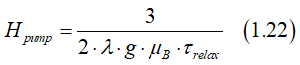
| Fig.7 Hall angle in similar devices (nanomagnets), which are fabricated in different parts of the same wafer. |
| Samples Volt 54B R66 (red) , L20 (green), L16 (blue). More samples details see here |
| click on image to enlarge it |
Figure 7 shows the data measured for three different nanomagnets fabricated at different parts of the same wafer. The 1st and 2nd derivatives (Fig.7 (b,c)) are nearly the same for these nanomagnets indicating that the ISHE contribution and consequently the spin polarization are the same in these nanomagnets. However, the αHE (Fig.S3 (a)) and consequently the αAHE are different for each nanomagnet. It shows that there is a parameter, which influences the AHE contribution, but does not influence the ISHE contribution and the spin polarization, and this parameter is different for each of these three nanomagnets.
Additionally, the perfect matching of derivatives for different nanomagnets excludes the possibility of existence of any magnetic domains, because the movement of the domain wall should be individual and different for each nanomagnet due to different distributions of fabrication defects, edge irregularities, and a slight difference in shape of the nanomagnets.
(note) In general, there are nanomagnets with different αISHE and consequently of different spin polarization on the same wafer. That depends on the quality of growth and nanofabrication. See details for each sample here. Fig.7 shows a general case for a relatively-good sample (a low number of defects and shape irregularities).
(proof 2:) ![]() Measurement at different current density
Measurement at different current density
Independence of ISHE from AHE |
| Measurement at different current density |
|---|
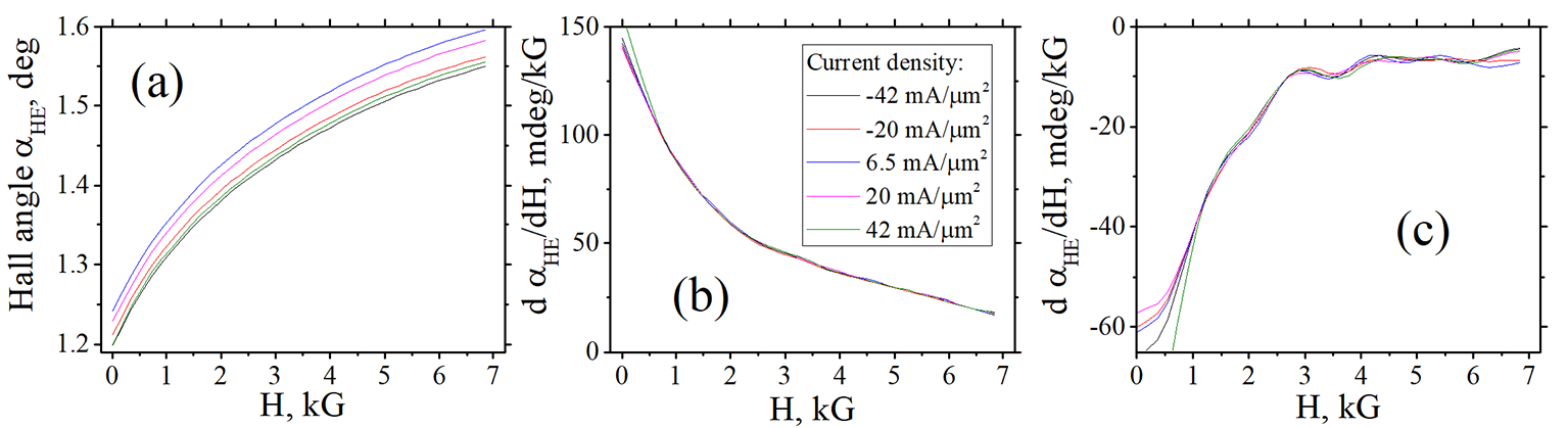 |
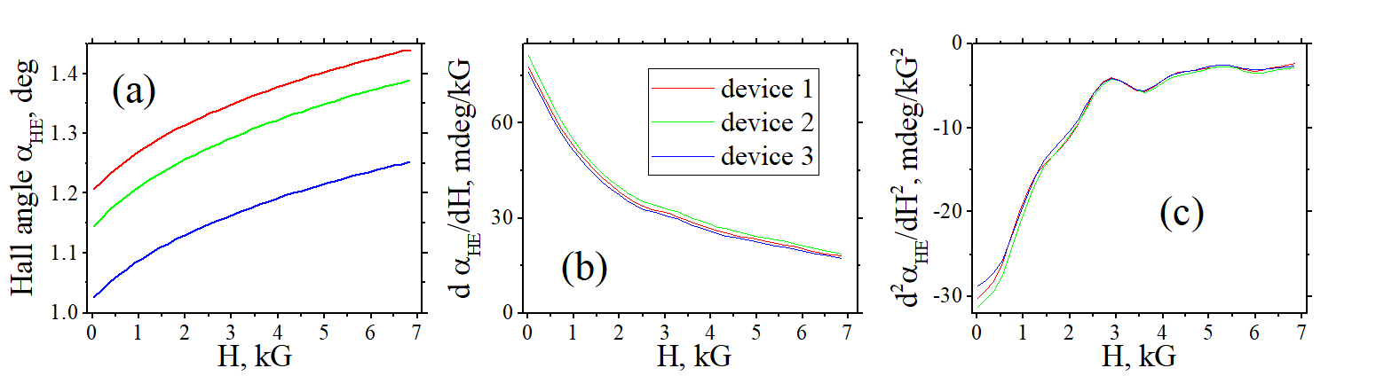
| Fig.8 Hall angle measured in the same device at different current densities |
| click on image to enlarge it |
Figure 8 shows the data measured at a different current density. The used current density is relatively high and the heating of the nanomagnet is expected. The heating was confirmed from the measured reduction of conductivity of the nanomagnet. The heating is not sufficient to change the ISHE contribution and therefore the spin polarization (Fig.8(b,c)). However, the AHE contribution is clearly reduced with the heating (Fig.8(a)). It again confirms the existence of a parameter, which influences the AHE contribution, but does not influence the ISHE contribution and the spin polarization.
(note) In general, there are nanomagnets, in which t αISHE depends on the current density. See details for each sample here. Fig.8 shows just one typical case.
 See the influence of Hall angle by the Spin- Orbit torque (SOT) here. The SOT describes the dependence on current polarity
Experiment. Measurement of dependence AHE and ISHE |
 |
| MMM 2020 conference |
| click on image to play video |
My presentation on this topic no MMM 2020 conference
Yes.
Not yet. For calibration of my magneto- transport probe, I am measuring the Hall effect in a thick (30 nm) Ta or Ru nanowire. The dependence of the Hall angle vs H is very linear. It seems to be the major contribution is from the Ordinary Hall effect.
In non-magnetic metal, the HS is substantially larger than in a ferromagnetic metal due to faster spin relaxation rate. As a result, 1st derivative of ISHE is much smaller than the OHE contribution (See Fig.4d) and therefore this makes it difficult to distinguish between the ISHE and OHE contributions.
Decomposing of measured hysteresis loop of the hall angle into its 3 contributions |
||
|
||
click on image to enlarge it |
(about another possible Hall effects) ![]()
The symmetry of the Hall effects limits possible contributions to a few possible contributions. Except AHE, OHE, ISHE, any other contribution should be at least 2 orders smaller. This fact is explained from the symmetry of the Hall effect. Any possible contribution to the measured Hall angle should obey two symmetry requirements: (1st symmetry requirement) : The Hall angle is linearly proportional to the electron current and therefore to the number of the conduction electron. The Hall angle should depend linearly at least on some property of conduction electron. (2d symmetry requirement) The Hall angle reverses its polarity when all the external magnetic field, the total spin of localized electrons and the total spin of conduction electrons are reversed. There is no other object or field in nanomagnet, which has the similar time- reverse symmetry. The Hall angle should depends linearly on each of theses objects or a 3d order of their product. Since the Hall angle is small (< one degree), a 3d order product is very small. There are only three possible contributions, which satisfies these symmetry requirements:
(1st contribution) Ordinary Hall effect, which is linearly proportional to external magnetic field H and wave vector of a conduction electron. The origin of this contribution is the Lorentz force.
(2nd contribution) Inverse Spin Hall effect, which is linearly proportional to the total spin of the conduction electrons Sconduct and therefore to the number of the spin- polarized conduction electrons. The origin of this contribution is the spin- dependent scatterings of spin- polarized electrons such as a screw scattering, side- jump scatterings and a scattering across an interface. The probability of these scatterings depends on the spin direction of conduction electrons, but not on the spin of the localized electrons.
(3d contribution) Anomalous Hall effect, which is linearly proportional to the total spin of localized electrons Slocal and the orbital moment of conduction electrons. Since spins of localized electrons is already aligned along the easy axis, the contribution is independent of the external magnetic field applied along the easy axis.
The symmetry restrictions, which limit the possible contributions to the Hall effect, can be understood as follows. A reversal of a sufficiently large external magnetic field causes the reversal of spins of localized, reversal of spins of conduction electrons and , as a result, the reversal of sign of the Hall angle αHall
![]()
where H is external magnetic field,Slocal is the total spin of localized electrons and Sconduct is the total spin of conduction electrons
From Eq.(8.1), the Hall angle should be the linear sum of each time- reversal parameter, which is describes as
![]()
Fig.6 shows how a hysteresis loop of measured Hall angles is decomposed into the sum of different contributions.
A nanomagnet with a strong PMA is a unique object, in which individual contribution of only 3 types of the Hall effects can be separated. Nowadays many new names of the similar Hall mechanism have appeared and this is a confusing issue. In fact, there are not so many "the Hall effects", which may exist. The symmetry does not allow it.
The different mechanisms should be distinguished and separated only based only on some experimentally distinguishable property or effect. There are not so many of those in a nanomagnet.
The first distinguish feature of Hall effect is the free parameter, on which the Hall effect depends. The free parameter should be magnetic. In case of our nanomagnet, there are only 3 such parameters: (parameter 1): external magnetic field H; (parameter 2): the total spin Slocal of localized electrons; (parameter 3) the total magnetic moment Sconduc of conduction electrons. Only these three magnetic parameters can be changed independently. Any external distortion of the magnetic system of nanomagnet can always be described as a sum of changes of these 3 free parameters.
According to these 3 free magnetic parameters, the 3 mechanisms of the Hall effect can be distinguished: OHE, AHE and ISHE.
The second distinguish feature of Hall effect is the even or odd symmetry with respect to a reversal of magnetic field when (H, Slocal , Sconduc) --> (-H, - Slocal, - Sconduc).
In our standard DC measurement, we measure only the odd contribution:
aOHE(-H)= - aOHE(H)
aAHE(-Slocal)= - aAHE(v)
aISHE(-Sconduc)= - aISHE(Sconduc)
Since are independent free parameters, the total even Hall angle can be divided into a sum of three contributions:
aHall(H, Slocal , Sconduc)= aOHE(H)+ aAHE(-Slocal) + aISHE(-Sconduc)
Next- order contribution can only be of 3rd order like H3, H2∙ Sconduct, H2∙Slocal, etc., which are much smaller and can be ignored.
The independence of parameters means that we can change one parameter without affecting another parameter. For example, we can inject externally the spin polarized conduction electron without affecting the spins of localized electrons. Or we can apply an external magnetic field plus the spin injection of the opposite spins. As a result, the spin polarization is not changed.
Even types of Hall effect. (not measured in our standard DC measurement setup)
For even type Hall effects:
aHall(-H, -Slocal , -Sconduc)= aHall(H, -Slocal , -Sconduc)
Obviously, the even type Hall effects is proportional to H2, H∙ Sconduct, H∙Slocal etc. An example of the even Hall effect is so-called the Planar Hall effect. Since we do not measure the even contribution, we do not discuss it.
In absence of other independent free magnetic parameters, the OHE, AHE and ISHE are only possible odd mechanisms of the Hall effect.
For example, let us consider the Hall effect in a non-magnetic metal covered by a ferromagnetic isolator. The magnetization of the isolator may be considered as a free parameter and a new mechanism of the Hall effect can be assigned. However, it is incorrect to do it. The magnetization in the isolator aligns the spins of localized and conduction electrons in the non-magnetic metal and therefore induces the AHE and ISHE. Even one give a new name of this Hall effect, it is still AHE + ISHE.
(about unambiguous evaluation of spin polarization) At the moment, I do not want to speculate about the absolute value of spin polarization.
However, it might be possible to trace whether the spin polarization increases or decreases from a sample to a sample or under a gate voltage (VCMA effect) or when current polarity is changed (SOT effect). The change of the spin polarization can be traced from the change of the 1st and 2nd order derivatives
The 1st and 2nd order derivatives should be larger when the equilibrium spin polarization is smaller. E.g. if the equilibrium spin polarization is 95 %, it can increase under a magnetic field maximum to 100 % and therefore the change is small. In contrast, if the equilibrium spin polarization is 5 %, the change to 100 % is large and . The 1st and 2nd order derivatives should be larger. The analysis is still no as simple, because derivatives also depend on the value of the spin relaxation. (See Fig.4 )
(about intrinsic magnetic field) There is an intrinsic magnetic field in a nanomagnet and it is influence the spin polarization of nanomagnet. However, it is difficult to estimate the value of the intrinsic magnetic field by this method, because additionally to the intrinsic magnetic field, the equilibrium spin polarization depends on the rate of the spin relaxation, the strength of the sp-d exchange interaction between conduction and localized electrons and the scattering rate between conduction and localized electrons.
In fact, one fitting parameter of experimental data is some sort of a magnetic field, which we assigned as HS. The fitting gives unambiguously the value of this magnetic field HS. The evaluated magnetic field HS is not related to intrinsic magnetic field. The HS describes the effectiveness of alignment of spins of the conduction electrons along the external magnetic field. The smaller HS is, the more effective alignment is. The spin alignment is less effective when the spin relaxation is faster. The spin alignment is more effective when spin precession damping is faster and therefore the Gilbert damping constant is larger.
The equilibrium spin polarization PS,0 does depend on the intrinsic magnetic field. However, it also depends on the strength of the sp-d exchange interaction between conduction and localized electrons and the scattering rate between conduction and localized electrons. Therefore, it is difficult to distinguish the sole contribution of the intrinsic field.
There are more direct methods of the intrinsic magnetic field than the described method. For example, we have developed another measurement method, in which it is possible to evaluate the strength of the intrinsic magnetic field. The method is based on a measurement of the strength of the perpendicular magnetic anisotropy (PMA). See .
The idea of the measurement can be explained in short as follows. In our nanomagnet the PMA has an interfacial origin. The PMA is due to the spin- orbit interaction (SO), which is enhanced at the interface. The SO by itself cannot break the time- inverse (TI) symmetry and therefore the SO requires an external magnetic field to break the TI symmetry. Only in the presence of an external magnetic field, the SO can manifest itself. As a result, the strength of the SO and therefore PMA is proportional to the total magnetic field, which electrons at interface experience. The total magnetic field is the sum of the intrinsic and external magnetic fields. From a measurement of the PMA strength as a function of the external magnetic field, the intrinsic magnetic field can be estimated. The intrinsic magnetic field includes the demagnetization field.
The strength of the PMA is characterized by the anisotropy field Hanis. We measure the as Hanis function of a perpendicularly- applied external magnetic field Hz. Figure shows the measured dependence. Since the Hanis increases a few times under Hz=7 kG, we conclude that the applied external magnetic of about 7 kG is comparable to the intrinsic magnetic field.
The intrinsic magnetic field is different from a nanomagnet to a nanomagnet, but it is within range of a few kGauss.
Experimental proof on absence of static domains in a nanomagnet |
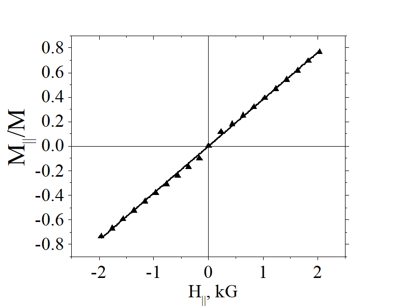 |
Linear dependence of in-plane magnetization vs. in-plane magnetic field. In this measurement, an external magnetic field is applied in plane (along the magnetic hard axis). The magnetization turns towards the in-plane field. The dependence of the in-plane component of the magnetization vs H is a perfect line, which is only possible when the nanomagnet is in a single- domain state. The linear dependence proves that the magnetization turns as whole (as a mono domain) towards the magnetic field instead of a movement of domain wall across nanomagnet as it would be in case of existence of a static domain. |
| click on image to enlarge it |
(about a perfect alignment of magnetization in a nanomagnet) There are several proofs, but I would like to mention 2
(experimental proof 1: linear dependence of M|| vs. H||): In this measurement (details here and here) an external magnetic field H|| is applied in plane (along the magnetic hard axis). The magnetization turns towards the in-plane field. The dependence of the in-plane component of the magnetization M|| vs H is a perfect line, which is only possible when the nanomagnet is in a single- domain state.
(proof of perfect alignment): In the case if some region has magnetization different from the perpendicular, the in-plane magnetic field H|| expands this region in order to minimize the magnetic energy and the dependence is substantially different from linear.
(experimental proof 2: existence of a nucleation domain in process of magnetization reversal ): The experimental measurements of thermally- activated magnetization switching in the same nanomagnets confirms that the magnetization switching mechanism of the studied nanomagnets is the nucleation- domain type. A nucleation domain is an unstable magnetic domain, which exists for a very short time (~a few milliseconds) during magnetization switching. The very existence of the nucleation domain confirms that the sample is mono domain because such nucleation domain can exist only in a single domain nanomagnet in absence of a static domain. Additionally, the size of nucleation domain is measured to be between 40 nm and 90 nm for our FeB and FeCoB nanomagnets (details are here and here). Such measurement is impossible in case when there are static domains.
(proof of perfect alignment): the nucleation domain can exists and therefore be measured in a single- domain nanomagnet. Otherwise, the pre- existed region of different magnetization just expands instead of creation of a nucleation domain.
(experimental proof 3: The stable static domain is at least a few times larger than the unstable nucleation domain. We have exactly similar result (even the measured signal is noisier) for a very small nanomagnets (d<50 nm), which size is even smaller than size of nucleation domain. The existence of a much larger static domain in such a small nanomagnet is absolutely impossible.
(proof of perfect alignment): there is a minimum size of static domain. When the size of nanomagnet is smaller that this size, there is no static domains
(about a possibility of usage of the method for a ferromagnetic film and a disturbance due to a static domain). Existence of static domains in in a planar film or bulk ferromagnet makes very difficult to use this method.
(magnetic domains of a ferromagnetic film) In a ferromagnetic film or in a bulk ferromagnet,, the magnetization monotonically increases with H due to a motion of domain walls. In a magnetic field the magnetic domains are smoothly rearranged in an increasing magnetic field making larger area of domains of magnetization along magnetic field. As a result, the magnetization is monotonically increases in a magnetic field. A modern Kerr microscope has an option, which allows to see magnetic domain distribution and redistribution while measuring a hysteresis loop of Kerr angle. This fact can be easily verified.
(magnetization of a single-domain nanomagnet) When the size of nanomagnet becomes smaller than the size of a magnetic domain, all spins of localized electrons are aligned in one perpendicular direction and the state of the nanomagnet becomes the single-domain state.
The reason why all spins of localized electrons are perfectly aligned in a nanomagnet in one direction can be understood as follows. For existence of a static magnetic domain, the positive exchange energy of a domain wall should be balanced by a negative magneto- static energy between dipoles of opposite magnetizations. When shape of nanomagnet is a circle with radius R and domain wall passes through its center, the magneto- static energy is proportional to domain area (~R2) and domain wall energy is proportional to its length (~R). When the size of nanomagnet decreases (decrease of R), the magneto- static energy decreases faster, at some size it becomes unable to balance the domain wall energy and nanomagnet state becomes a single- domain state.
 Video
Video 
Measurement of Anomalous Hall effect, Inverse Spin Hall and spin polarization of conduction electron
Conference presentation.MMM 2020 |
|---|
![]()
![]() I am strongly against a fake and "highlight" research
I am strongly against a fake and "highlight" research ![]()
![]()
![]()
![]()
![]()
![]()
I will try to answer your questions as soon as possible