Dr. Vadym Zayets
v.zayets(at)gmail.com
My Research and Inventions
click here to see all content |

Dr. Vadym Zayetsv.zayets(at)gmail.com |
|
|
more Chapters on this topic:IntroductionTransport Eqs.Spin Proximity/ Spin InjectionSpin DetectionBoltzmann Eqs.Band currentScattering currentMean-free pathCurrent near InterfaceOrdinary Hall effectAnomalous Hall effect, AMR effectSpin-Orbit interactionSpin Hall effectNon-local Spin DetectionLandau -Lifshitz equationExchange interactionsp-d exchange interactionCoercive fieldPerpendicular magnetic anisotropy (PMA)Voltage- controlled magnetism (VCMA effect)All-metal transistorSpin-orbit torque (SO torque)What is a hole?spin polarizationCharge accumulationMgO-based MTJMagneto-opticsSpin vs Orbital momentWhat is the Spin?model comparisonQuestions & AnswersEB nanotechnologyReticle 11
more Chapters on this topic:IntroductionTransport Eqs.Spin Proximity/ Spin InjectionSpin DetectionBoltzmann Eqs.Band currentScattering currentMean-free pathCurrent near InterfaceOrdinary Hall effectAnomalous Hall effect, AMR effectSpin-Orbit interactionSpin Hall effectNon-local Spin DetectionLandau -Lifshitz equationExchange interactionsp-d exchange interactionCoercive fieldPerpendicular magnetic anisotropy (PMA)Voltage- controlled magnetism (VCMA effect)All-metal transistorSpin-orbit torque (SO torque)What is a hole?spin polarizationCharge accumulationMgO-based MTJMagneto-opticsSpin vs Orbital momentWhat is the Spin?model comparisonQuestions & AnswersEB nanotechnologyReticle 11
|
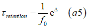
Thermally-activated magnetization switching. Measurements of coercive field, retention time, Δ Spin and Charge TransportAbstract:
A magnetic material has two stable magnetization directions. An external magnetic field may switch the magnetization between these two states. The magnetic field, at which the magnetization is switched, is called the coercive field Hc. This magnetization switching is a thermally- activated process. Therefore, it depends on temperature and is assisted by thermal photons, phonons and magnons. Because of its thermal nature, the magnetization switching is probabilistic. It means that for each scan of a magnetic field, the magnetization switching occurs at a slightly-different magnetic field.In most cases, the magnetization switching is initialized by a magnetization reversal in a very small area, which is called the magnetic domain, and the next expansion of the domain over all ferromagnetic material (over all nanomagnet). There are two types of the magnetic domains: the static magnetic domain, which is stable in time, and the nucleation domain, which is unstable and exists only for a very short time of about a few nanoseconds during the magnetization switching. Features of thermally activated switching of the magnetization are described. A new high-precision measurement method of the coercive field, retention time, Δ and the size of a switching nucleation domain is described below.
|
Measurement method of all parameters of thermo- activated switching (coercive field, retention time, parameter Δ, size of nucleation domain) |
 |
| main idea of measurement method: magnetization switching time is measured vs. applied magnetic field. The dependence of Log(switching time) vs magnetic field is linear. It makes the fitting very precise and allows to evaluate all switching parameters with a very high precision |
| In comparison with other method, only this method is free of systematic errors and allows to achieve a high- precision, high-repeatability and high- reliability. |
| (what is measured) |
| (which parameters are evaluated) |
| Click on image to enlarge it |
![]() Questions & Answers
Questions & Answers
-----------![]() (19) Questions & Answers
(19) Questions & Answers
 -------------------------------
![]() ..............
..............![]()
| Measurement method of coercive field, retention time, parameter delta, size of a nucleation domain |
|---|
 |
| (measurement method): |
| (thermally-activated switching): |
| (features of the method): high precision; high repeatability, high reliability |
Note. I have developed this measurement method in 2017-2018 |
| click on image to enlarge it |
Existence of a coercive loop as indication of a thermally - activated process -> |
 |
| It doesn't matter whether the coercive loop is large or small, square - shaped or some complex shape, the existence of a coercive field is always due to a thermally- activated process |
| Existence of a hysteresis loop |
 The statement is applied to a micro- or nano- sized object (e.g. a domain, domain wall), in which the energy barrier comparable with the energy of a thermal fluctuation (~kT) The statement is applied to a micro- or nano- sized object (e.g. a domain, domain wall), in which the energy barrier comparable with the energy of a thermal fluctuation (~kT) |
| The statement is applied also to more complex measurements of thermally activated processes like FORC |
| click on image to enlarge it |
A thermal fluctuation may switch the magnetization of a nanomagnet between its two opposite stable directions.
A bit of recorded data of any magnetic memory can be destroyed due to unwanted thermally activated switching of the magnetization. The data storage time can be as short as a minute or can be as long as a billion years. Using the below-described measurement method, the data storage time can be measured with a very high precision in both cases.
In order to record a bit of data into a magnetic memory, the magnetization of one memory cell should be reversed. It is done by applying a recording magnetic film, which reverses the magnetization. The mechanism of the switching is a thermally activated magnetization switching.
![]()
![]() Understanding of features of a thermally activated magnetization switching is important for both the data and data recording of the magnetic memory!!!
Understanding of features of a thermally activated magnetization switching is important for both the data and data recording of the magnetic memory!!!
A. Yes. An irreversible magnetization reversal occurs after an event when the number of the electrons on the higher-energy spin-down level exceeds the number of electrons on the lower-energy spin-up level. Additionally, a thermally- activation, the magnetization reversal may occur due to a spin injection (see here) or a parametric- resonance (See here)
Thermal mechanisms of magnetization reversal. Quantum vs. classical descriptions
 Magnetization reversal occurs when:
(Quantum description): number of spin-down electrons exceeds the number of spin-down electrons
(Classical description): the electron moves over or tunnel through an energy barrier, which separates the spin-down and spin-up stable electron states. This means that the electron spins is inclined more than 90 deg with respect to its stable position by a thermally activated random magnetic field.
 Quantum description
In the quantum description the magnetization reversal is described as a quantum transition between the energy levels. Magnetization reversal occurs at a moment of time when the number of electrons on a higher-energy level exceeds the number of electrons on a lower-energy level.
Thermal mechanism of the magnetization reversal. Quantum description |
|||||||||
| In the quantum description the magnetization reversal is described as a quantum transition between the spin-up and spin-down energy levels. | |||||||||
|
|||||||||
| Magnetization reversal occurs when the number of spin-down electrons exceeds the number of spin-down electrons. As a result, the internal magnetic field reverses its direction and the spin-down state becomes a stable state. | |||||||||
| Blue ball shows the magnetization (the total spin) of the nanomagnet (or nucleation domain). Hint is the internal magnetic field, which is aligned either along or opposite to the magnetic easy axis (See details here). . Hext is the external magnetic field. Green balls are exchanged coupled spins of localized electrons. The angle of the magnetization precession depends on a relative number of spin-down and spin-up electrons (See here) | |||||||||
| Click on image to enlarge it |
![]() (fact about total spin) within a nucleation domain or a single-domain nanomagnet, directions of all spins are glued together by a very strong exchange interaction. The total spin or magnetization (shown as a blue ball) is the sum of spins of all localized electrons within the nucleation domain. At any time during magnetization reversal the magnitude of the total spin remains the same, the direction of the total spin changes. A nucleation domain should be considered as a single quantum object with a single spin.
(fact about total spin) within a nucleation domain or a single-domain nanomagnet, directions of all spins are glued together by a very strong exchange interaction. The total spin or magnetization (shown as a blue ball) is the sum of spins of all localized electrons within the nucleation domain. At any time during magnetization reversal the magnitude of the total spin remains the same, the direction of the total spin changes. A nucleation domain should be considered as a single quantum object with a single spin.
![]() (fact about required small size of nucleation domain) The larger the size of the nucleation domain is and, therefore, the larger the number of the spins is, the smaller the probability of thermally-activated magnetization reversal becomes.
(fact about required small size of nucleation domain) The larger the size of the nucleation domain is and, therefore, the larger the number of the spins is, the smaller the probability of thermally-activated magnetization reversal becomes.
![]() If the probability for a quantum transition from the spin-up to the spin down level for one electron equals p, then the probability for the transition of two electrons in the same time is p·p. The the probability for the transition of n- electrons in the same time is pn. If the volume of the ferromagnetic domain is Vdomain , the number of the spin in the domain is M ·Vdomain. Then, the probability of a reversal of the nucleation domain is
If the probability for a quantum transition from the spin-up to the spin down level for one electron equals p, then the probability for the transition of two electrons in the same time is p·p. The the probability for the transition of n- electrons in the same time is pn. If the volume of the ferromagnetic domain is Vdomain , the number of the spin in the domain is M ·Vdomain. Then, the probability of a reversal of the nucleation domain is
pdomain=pM ·V_domain
![]() (fact about the retention time) The longer the waiting time is, the larger the probability of thermally-activated magnetization reversal becomes.
(fact about the retention time) The longer the waiting time is, the larger the probability of thermally-activated magnetization reversal becomes.
 Classical description or Néel description
In the classical description the magnetization reversal is described as as a jump over or tunneling of an electron through the energy barrier, which separates two stable spin-up and spin-down states, which are separated by an energy barrier. The height of the barrier is lowered by an external magnetic field. When the magnetic field equals to the coercive field, the energy barrier bacomes sufficiently low for the electron to tunnel to another stable state.
Thermal mechanism of the magnetization reversal. Classic description |
| In the classic description the magnetization reversal is described as a jump over or tunneling of an electron through the energy barrier, which separates two stable spin-up and spin-down states.. |
| The green ball shows the magnetization direction, the arrows shows the strength and direction of the external magnetic field H . |
 |
| Magnetic energy as a function of the magnetization angle with respect to the magnetization direction. The energy is smallest when magnetization angle is along the easy axis (angle=0 and 180 deg). The energy minimums correspond to two stable magtization state. The energy maximums correspond magnetization direction perpendicular to the easy axis (along the hard axis). |
| The animation parameter is the strength of external magnetic field with respect to anisotropy field H/Hoff . When the external magnetic field is along magnetization the energy dip decreases. When the external magnetic field is opposite to magnetization the energy dip increases. |
(reversal mechanism) When the barrier height becomes sufficiently small, the magnetization interacts with an external particle. Due to this thermal process, the magnetization gains the energy and momentum to jump over the energy barrier and reverses own spin direction. |
| Click on image to enlarge it |
According to how the energy of perpendicular magnetic anisotropy (PMA) described, there are two classical descriptions:
(classical description 1): oversimplified Neel description
In this model the simplest dependency of the PMA anergy is assumed. This model does not fit all experimental data, but it is a good approximation in many cases
Magnetic energy: 
Energy barrier: ![]()
(classical description 2): full description based on properties of the spin-orbit interaction
This model correctly described all features of the perpendicular magnetic anisotropy (PMA).
Magnetic energy: 
Energy barrier: 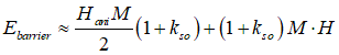
![]() (problem 1of classic description): quantum tunneling
(problem 1of classic description): quantum tunneling
![]() The classic description is based on tunneling through the energy barrier between 2 stable states. The quantum tunneling may occur only between two different quantum states, which are spatially separated. In contrast, the magnetization reversal means the spin reversal for one single quantum state. Only the degree of the broken time- inverse symmetry is changing during the magnetization reversal.
The classic description is based on tunneling through the energy barrier between 2 stable states. The quantum tunneling may occur only between two different quantum states, which are spatially separated. In contrast, the magnetization reversal means the spin reversal for one single quantum state. Only the degree of the broken time- inverse symmetry is changing during the magnetization reversal.
![]() (problem 2 of classic description): one electron tunnelin vs. magnetization reversal of whole nucleation domain
(problem 2 of classic description): one electron tunnelin vs. magnetization reversal of whole nucleation domain
![]() The tunneling occurs only for a single electron. However, the magnetization reversal occurs simuteneously for a whole nucleation domains, which contains billions of electrons (spins).
The tunneling occurs only for a single electron. However, the magnetization reversal occurs simuteneously for a whole nucleation domains, which contains billions of electrons (spins).
![]() (problem 3 of classic description): Large difference between anisotropy field and coercive field.
(problem 3 of classic description): Large difference between anisotropy field and coercive field.
![]() The anisotropy field is the magnetic field, at which the spin turns perpendiculary to the easy axis and whch corresponds to the top of the energy barrier. The coercive field is the magnetic field, at which the magnetization is switched. In a Fe nanomagnet, the anisotropy field may reach 10 000 Gauss when the coercive field may be only about 400 Gauss. It means that such a small coercive field reduces only slightly the hight of the energy barrier. Still it triggers the magnetization reversal.
The anisotropy field is the magnetic field, at which the spin turns perpendiculary to the easy axis and whch corresponds to the top of the energy barrier. The coercive field is the magnetic field, at which the magnetization is switched. In a Fe nanomagnet, the anisotropy field may reach 10 000 Gauss when the coercive field may be only about 400 Gauss. It means that such a small coercive field reduces only slightly the hight of the energy barrier. Still it triggers the magnetization reversal.
(note): There are 3 possible mechanisms of magnetization reversal: the mechanism of domain wall shifting and expansion of static domains; the mechanism nucleation and mechanism of single- domain magnetization reversal
(sample size -> reversal mechanism) ![]() The mechanism of magnetization reversal depends on the sample size. The reversal mechanism for a continuous film and a large sample is the domain wall shifting of static domain. The reversal mechanism for a sample of a moderate size (~ from 50 nm to 20 μm) is by a nucleation domain. The reversal mechanism for a smallest sample (<50 nm) is the single- domain reversal.
The mechanism of magnetization reversal depends on the sample size. The reversal mechanism for a continuous film and a large sample is the domain wall shifting of static domain. The reversal mechanism for a sample of a moderate size (~ from 50 nm to 20 μm) is by a nucleation domain. The reversal mechanism for a smallest sample (<50 nm) is the single- domain reversal.
mechanisms of magnetization reversal |
||||||||||||||||||||
| There are 3 distinguished mechanisms of the magnetization reversal: (mechanism 1) Domain movement of static domain. This mechanism is a feature of a large-size nanomagnet or a magnetic film, in which a static domain exists. (mechanism 2) Creation of a nucleation domain. This mechanism is a feature of a moderate-size nanomagnet, in which static domains do not exist and the equilibrium magnetization is homogeneous (magnetization is the same direction through all nanomagnet). When magnetic field is applied opposite to the magnetization, at first magnetization of a small area (nucleation domain)is reversed. Next, the area of the reversed magnetization expand over whole nanomagnet. (mechanism 3) Single-domain magnetization reversal. This mechanism is a feature of a smallest-size nanomagnet, which size is smaller the the size of the nucleation domain. As a result, the magnetization is reversed coherently over the whole nanomagnet. | ||||||||||||||||||||
|
||||||||||||||||||||
| Click on image to enlarge it |
samples: large-size nanomagnet, magnetic film
In this case there are static domains of two opposite magnetization directions. When magnetic field is applied, the domain wall slightly moves making the larger the area of domains of magnetization along magnetic field and the smaller the area of domains of the magnetization opposite to the magnetic field. As the magnetic field increases, the area of domain becomes larger and larger and correspondingly the area of opposite domain becomes smaller and smaller until it disappear. At each magnetic field the domain wall is pinned
samples: moderate-size nanomagnet
In this case the magnetization of the whole nanomagnet remains opposite to applied external magnetic field until the critical field (the switching field), at which the magnetization of small area (the nucleation domain) coherently reversed and becomes parallel to the external magnetic field. Immediately after that the domain wall moves expanding the nucleation domain over the whole sample. Main feature of this mechanism is that the domain wall is not pinned. At the moment, at which the nucleation domain is created, the domain wall moves without any obstacles until the magnetization of the whole nanomagnet becomes parallel to the applied magnetic field.
samples: smallest-size nanomagnet
In this case the magnetization of the whole nanomagnet remains opposite to applied external magnetic field until some critical field (the switching field), at which the magnetization of the whole nanomagnet rotates to become parallel to the external magnetic field. Through the whole switching process the magnetization at any point of the nanomagnet remains parallel. There is no any magnetic domains.
(magnetization reversal) mechanism 1a: movement of wall of static-domains |
||
|
||
| (left) hysteresis loop of nanomagnet (magnetic film) with static domains. (right) top view of a domain structure of the magnetic film. The whiter areas show area, where magnetization direction is to the left. The darker areas show area, where magnetization direction is to the right. Blue arrow shows the direction and magnitude of external magnetic field. Green arrow shows the direction and magnitude of the total magnetization of the film. | ||
| As magnetic field H increases, the domain walls move and domains of magnetization direction parallel to H increase until they cover all film. Because of domain pinning, the extension of the domain requires the energy. It is reason why the domain area extends gradually with increase of magnetic field and why the area is different parts of increase and decrease of H (the reason for the loop) | ||
(magnetization reversal) mechanism 1b: nucleation of a static domain following movement of wall (under increase of magnetic field) |
||
|---|---|---|
 |
||
| (left) measured Hall angle vs H for Co(0.6):Pt(10) ; (right) top view of a domain structure of the magnetic film. | ||
| There is no static domain at H=0. Static domains are nucleated at at a weak magnetic field. Next, static domain expand their volume as H increases. Above H2 the magnetization is parallel to H. | ||
| difference between magnetization-reversal mechanism 1b & 1a: (mechanism 1a) domain walls move at both the positive and negative magnetic field, because magneto-static energy of domains is high. (mechanism 1b) static domains are nucleated & domain walls move only when magnetic field is opposite to the magnetization, because magneto-static energy of domains is low. | ||
| mechanism 1b-> a thinner film. mechanism 1a-> a thicker film. | ||
| Click on image to enlarge it |
A. It is because of the size dependence of the magnetostatic interactions.
(exchange interaction vs. magnetic-dipole interaction). There are two interactions between spins of different electrons. The short-range very-strong exchange interaction and the long-range moderate (low)-strength magnetic-dipole interaction. In a ferromagnetic metal, the exchange interaction aligns atoms parallel to each other. The dipole interaction aligns spins opposite each other. Even though it is very strong, the exchange interaction exists only between electrons of neighboring atoms and, therefore, the exchange interaction does not accumulate with an increased number of atoms. For a small number of atoms, the exchange interaction aligns all spins to be parallel. When the number of atoms increases, the exchange interaction remains unchanged, but dipole interaction is accumulated and, therefore, increases. When the number of atoms exceeds some critical number, all spins within a part of the nanomagnet reverse their direction and a magnetic domain is formed. The balance between the magnetostatic interaction and the exchange interaction determines the size of the magnetic domain.
(domain volume vs domain-wall) The magnetic energy is proportional to the number of spins and, therefore, to the volume of the magnetic domain. In contrast, the energy of the domain wall is proportional to the surface area of the domain. The balance between the magnetic volume energy and the domain- wall determines the sizes and distribution of the magnetic domains.
When the nanomagnet size is smaller than the minimum domain size, the nanomagnet is in a single-domain state.
The strength of the exchange and the dipole interactions, the number of imperfections and defects in both inside of the nanomagnet volume and at the nanomagnet surface, all substantially influence the domain size.
A. In order to reverse its spin, an electron should interact with a non-zero- spin particle like a photon or a magnon. For example, if the probability to reverse the spin of one electron equals p, then the probability to reverse the spin of two electrons is smaller and equals p·p. The probability to reverse the spin of n- electrons is even smaller and equals pn. Therefore, the probability is higher to reverse a smaller amount of the spins.
A. In a ferromagnet, directions of all spins are glued together by very strong exchange interaction. It is impossible to reverse only one spin. The energy of the domain wall would be too large. It requires some amount of spins so that the dipole interaction overcomes the energy of the domain wall. It determines the minimum size of the magnetic domain or, the same, the minimum amount of the spins, which can be simultaneously reversed.
The magnetization M of a ferromagnet is defined as a number of the spins per the ferromagnet volume. If the volume of the ferromagnetic domain is Vdomain , the number of the spin in the domain is M ·Vdomain. Then, the probability of a reversal of the nucleation domain is calculated as (see previous question)
pdomain=pM ·V_domain
Therefore, the probability of switching is proportional to the volume of the nucleation domain.
A. The static domains are stable. In the case of static domains, there is a balance between magnetostatic and exchange energies. At different external magnetic field, the size of domains changes, but always the balance is possible. The balance can exists for a relatively large nanomagnet, which area is sufficient to fit several large-area domains.
The nucleation domain is not stable. For the nucleation domain the balance between magnetostatic and exchanges energies cannot be achieved. It is the case of a small nanomagnet, in which magnetostatic is smaller the domain wall energy for any possible domain configuration. As a result, it is energy favorable to remove domain wall to minimize the exchange energy since the magnetostatic energy has a small contribution. Therefore, as soon as a nucleation domain is formed, its domain wall immediately expands over whole nanomagnet.
A. It is because at any applied external magnetic field there is a balance between magnetostatic and exchanges energies. For each value of the external field, there is an optimum domain size for the balance.
E.g. let us consider bubble domains of the circle shape and radius R in a thin film. The magnetostatic energy is roughly proportional to the area of domain (~R2 · EMS), the energy of domain wall is proportional to length of the domain wall (~R· EEX) and the energy of magnetic interaction with magnetic field is is roughly proportional to the area of domain (~R2 · EH· H). When the external magnetic field increases, the radius of the bubbles domains becomes larger. As a results, the energy of domain wall increases and the magnetostatic energy decreases. At any field there is a balance: R2 · EMS- R· EEX - R2 · EH· H =constant
(main reason for an expansion of a magnetic domain (a movement of a domain wall):)
A domain wall moves when the total energy decreases for a larger domain size. It is always the case for a single domain nanomagnet, because the dipole interaction in a single domain nanomagnet is insufficient to stabilize a two- domain state. However, sometimes the domain wall may be stopped and stick to a defect or an imperfection (domain-wall pinning).
(Expansion of a static domain): At each value of the external magnetic field H, it should be a balance between magnetic energy of interaction of magnetic field with magnetization of each domain, energy of domain walls and dipole interaction. This balance determines the sizes of static domains.
A. It is because the energy barrier between single-domain and nucleation domain states is smaller than the energy barrier between two single-domain states of opposite magnetization. The energy barrier is proportional to the area of the nucleation domain (See here) and becomes smaller as the size of the nucleation domain is reduced
samples: large-size nanomagnet, magnetic film
citation from
| Fig. 1 (part) from |
Part 2.1 pp.362
"The connection between microstructural defects and magnetic properties has long been known, and the common terminology for magnetic materials as “hard” and “soft” stems from this [16]. Increased concentration of dislocations in single crystal ferromagnetic metals results in increased major loop coercivity and decreased initial and reversible susceptibilities [3,17]. The initial magnetization curve (i.e., from a demagnetized state) of a ferromagnet can be seen schematically to be divided into three stages under external field H before saturation (Fig. 1). The initial stage (low applied fields) involves reversible domain wall displacement and bowing (Fig. 1(a) and (b)). The domain wall will return to its initial position if the external field is removed (Fig. 1(a)). The domain wall is pinned by some dislocations or other defects (black spots) in this stage (Fig. 1(b)) and then bends due to the applied field. At higher fields the domain wall breaks away from the defects and the magnetization jumps discontinuously, generating Barkhausen noise [18]. The domain with the easy axis magnetization vector having a component in the same direction as the applied field direction grows (Fig. 1(c) and (d)). Ultimately and ideally, the material will consist of a single domain (Fig. 1(e)) at the end of the second stage. Finally, in the third stage at the highest applied fields, the domains will rotate away from their magneto crystalline easy axis to align with the external field and the magnetization becomes saturated (Fig. 1(f)). Processes (a) to (b) can be seen as reversible, as domain walls have not moved through pinning defects. Similarly, processed (e) to (f) are reversible, as it is just a rotation of the magnetic moment. These reversible processes generate what is known as the defect-free or an hysteretic magnetization [18]. Processes (c) to (d), however, are irreversible and result in hysteresis, as they involve the magnetization moving over an energy barrier (the pinning defect), discontinuously acquiring magnetization energy. It is apparent, then, that the character of the defects (concentration, size, shape, and magnetic nature) will affect the domain wall pinning and thus the processes in the (c) to (d) region. A higher defect concentration should lead to a smaller slope in magnetization in this region (i.e., a higher field is required to advance the magnetization by a given amount). Note that a similar argument can be made with consideration of a major hysteresis loop, rather than an initial magnetization curve as was described here. In principle, then, a given set of defects in a magnetic material should result in characteristic hysteresis behavior when evaluated in a range of field histories, such as with major and minor loops and FORCs. These same defects generate Barkhausen noise due to discontinuous jumps in magnetization as domain walls move past defects, and thus a simulation containing the effects of defects on hysteresis should be able to predict the Barkhausen noise spectrum generated as part of a NDE measurement of a magnetic steel"
Magnetization reversal due to domain- wall movement of static domains. Two mechanisms. |
|||||||||||||||
|
|||||||||||||||
| Additional loop features may exist when there is no static domain without magnetic field and static domains are nucleated under magnetic field applied opposite to the magnetization (See Fig. 1b above) | |||||||||||||||
| Click on image to enlarge it |
![]() (mechanism 1: reciprocal)
(mechanism 1: reciprocal)![]() :Magneto-static
:Magneto-static
Domain wall moves in order to decrease the magneto-static energy. The area of domain, which magnetization is along to external magnetic field, becomes larger. The area of domain, which magnetization is opposite to external magnetic field, becomes smaller. There is no coercive field for this mechanism. The change of the total magnetization is smooth and continuous with increase of the external magnetic field. The change is fully reversible. The mechanism is time- independent.
![]() (mechanism 2: non- reciprocal)
(mechanism 2: non- reciprocal) ![]() : Thermo- activation
: Thermo- activation
When the domain wall is moving, it can stick to a fabrication defect or a border irregularity. The domain wall overcomes such energy barrier by a thermo-activation mechanism. It means it assisted by a thermo fluctuation. The change of the total magnetization is step-like with some coercivity. The change is irreversible. The mechanism is time- dependent. It means that the probability of a thermo fluctuation, which assists the domain wall to overcome the energy barrier, is higher for a longer waiting or measuring time (as for any thermo- activated switching)
![]()
![]()
![]()
![]() Two types of magnetic domains:
Two types of magnetic domains:
The static domains exist even without any external magnetic field (See fig. 1(a)) or under a bias magnetic field fig. 1(b).
The hysteresis loop of a sample having static domains is smooth and does not have step-like features.
A nucleation domain exists for a very short moment during the event of the magnetization reversal. As soon as a nucleation domain is created, its domain wall moves expanding the domain over the whole sample.
The hysteresis loop of a sample having a nucleation domain has step-like features.
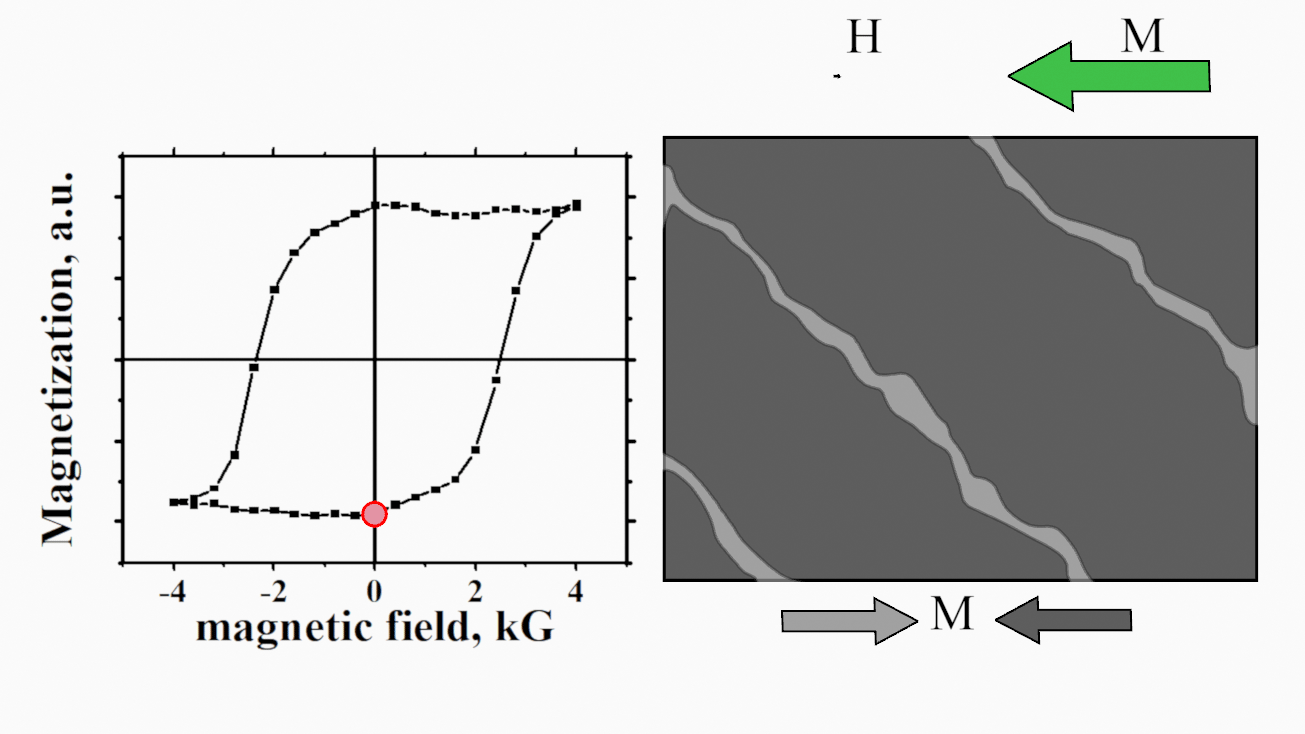
Figure 1 shows the schematic diagram of a hysteresis loop of a ferromagnetic nanomagnet. It shows the dependence of the nanomagnet magnetization M on the applied magnetic field. The magnetic field is scanned from a negative to positive value and back to negative. In the case of a sufficiently large magnetic field, the magnetization is always aligned along the magnetic field. However, at a smaller field just after a reversal of the external magnetic field, the magnetization does not follow the reversal and remains in the opposite direction to the magnetic field until the magnetic field reaches the threshold field, at which the magnetization is reversed to be again parallel to the external magnetic field. The threshold magnetic field, at which the magnetization is reversed, is called the coercive field Hc (See Fig.1).
A hysteresis loop for the magnetization switching exists for the following reason. The state, in which the magnetization is opposite to the direction of an external magnetic field, is in an unstable equilibrium. The state, in which the magnetization is parallel to the magnetic field, is more energetically favorable. However, there is an energy barrier between the "up" and "down" magnetization states and the magnetization reversal may occur only when the magnetization overcomes the barrier. The assistance of a thermal fluctuation is required in order to overcome the energy barrier. Because of the critical dependence of the reversal event on the existence of a thermal fluctuation, this type of magnetization reversal is called thermally-activated magnetization switching. The properties of the thermally-activated magnetization switching are important for magnetic data recording and magnetic data storage.
There is an energy barrier between two stable states, when the magnetization is parallel and antiparallel to the external magnetic field. The magnetization can overcome this barrier only with assistance of a thermal fluctuation.
Two methods to measure Hc: switching time or switching field |
||||||||||||
|
||||||||||||
| There is an energy barrier Ebarrier between up- and down-magnetization states. A thermal fluctuation assists the to overcome the barrier and to reverse direction | ||||||||||||
| Two method to overcome Ebarrier : (1) make Ebarrier lower. (2) wait for a thermal fluctuation of a higher energy. | ||||||||||||
| (method 1 to reverse magnetization): increase magnetic field. It makes the energy barrier between two states smaller. | ||||||||||||
| (method 2 to reverse magnetization): wait a longer time. It the probability of a required higher-energy thermal fluctuation higher. | ||||||||||||
| Click on image to enlarge it |
(method 1) ![]() Increase magnetic field.
Increase magnetic field.
The external magnetic field lowers the height of the energy barrier and makes the probability of a magnetization reversal higher. When the increasing magnetic field reaches Hc, the barrier height becomes sufficiently low and the magnetization is reversed.
(method 2) ![]() wait a longer time.
wait a longer time.
A thermal fluctuation of a higher energy is required to overcome a higher energy barrier. Waiting for a longer time makes the probability of the required higher-energy fluctuation greater.
![]() Methods of either applying a stronger magnetic field or waiting a longer time both lead to the magnetization reversal. For example, the reversal probabilities may be equal for the cases when the field is smaller but the waiting time is longer or when the field is larger but the waiting time is shorter.
Methods of either applying a stronger magnetic field or waiting a longer time both lead to the magnetization reversal. For example, the reversal probabilities may be equal for the cases when the field is smaller but the waiting time is longer or when the field is larger but the waiting time is shorter.
Hysteresis loop of a multi particle system or a magnetic film with static domains |
 |
| Fig. 2 The hysteresis loop is not of the rectangular shape as in the case of nanomagnet (Fig.1) . Fig is from here |
| Click on image to enlarge it |
case 1: (a multi particle system): It consists of many nanomagnets. The magnetization of each nanomagnet is reversed at a slightly different magnetic field. It makes the gradual change of the average magnetization.
case 2: (a magnetic film with complex domain structure): Between two states, when the magnetization is fully parallel to the external field, there is a state of complex domain structure. The amount of domain area is changed as the external magnetic field changes. It makes the gradual change of the average magnetization.
case 3: (intermediate magnetization direction): Additionally to the two states, when the magnetization is parallel and antiparallel to the external magnetic field, there might be additional intermediate state of local minimums of magnetic energy, when the magnetization is at some angle (between 0 and 180 deg) with respect to the magnetic field.
 Statistical nature of the thermally- activated magnetization switching
The thermally- activated magnetization switching is statistical process. It is described by statistical parameters and formalism like the average and statistical distribution.
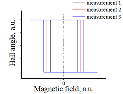
Every time you measure, the magnetic field of the magnetization switch
(single-shot measurement) ![]() Don't do a single-shot measurement for parameters of thermally- activated magnetization switching like Hc
Don't do a single-shot measurement for parameters of thermally- activated magnetization switching like Hc
Magnetization switching -> thermally- activated process |
Coercive field -> dependance on measurement time |
 |
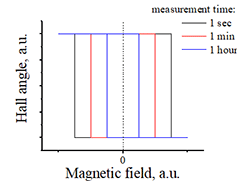 |
| Fig.8. Each time the switching of magnetization occurs at slightly different magnetic field. Click on image to enlarge it | Fig.9 The longer the scan of magnetic is, the shorter the coercive field is. |
![]() fact 1: Since the magnetization switching is a thermally- activated process, the distribution of switching fields is described by the thermal statistics
fact 1: Since the magnetization switching is a thermally- activated process, the distribution of switching fields is described by the thermal statistics
Average of the switching field is defined as the coercive field.
![]() fact 2: The longer the scan of magnetic field is, the shorter the coercive field is.
fact 2: The longer the scan of magnetic field is, the shorter the coercive field is.
Figure 3 explains this fact. When a magnetic field is applied opposite to the magnetization direction, for a while the magnetization is wiggling around its direction. next, it turns along magnetic field. The average magnetization-reversal time is fixed and it is proportional to the applied magnetic field.
|
||||||||
| From this measurement, all parameters of thermally -activated switching ( Hc, τreten , Δ and size of a nucleation domain) are evaluated with a |
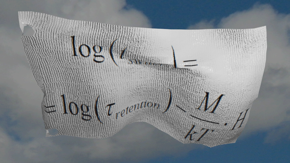
 In this method dependence of the magnetization switching time on the external magnetic field is measured. From this measurement, coercive field Hc, retention time τreten, parameter delta Δ and size of a nucleation domain for magnetization reversal.
![]()
![]()
![]() The magnetization switching time was measured as follows. A magnetic field H was applied opposite to the magnetization direction and the time interval, after which the magnetization is reversed, was measured. The measurement was repeated 200 times and a statistical analysis was applied to find the average of tswitch. Figure 10 shows the measured tswitch as a function of the magnetic field. On a logarithmic scale, the magnetization switching time is linearly proportional to the magnetic field as it is predicted by the Néel model of thermally activated magnetization switching
The magnetization switching time was measured as follows. A magnetic field H was applied opposite to the magnetization direction and the time interval, after which the magnetization is reversed, was measured. The measurement was repeated 200 times and a statistical analysis was applied to find the average of tswitch. Figure 10 shows the measured tswitch as a function of the magnetic field. On a logarithmic scale, the magnetization switching time is linearly proportional to the magnetic field as it is predicted by the Néel model of thermally activated magnetization switching
![]() Detailed steps of a measurement of dependence of magnetization switching time on the magnetic field (Fig.10 )
Detailed steps of a measurement of dependence of magnetization switching time on the magnetic field (Fig.10 ) ![]() :
:
(step 1) ![]() (reset of the magnetization): Applying a large magnetic field. The magnetization of the nano magnet is fully saturated. There no domain or pinned domain.
(reset of the magnetization): Applying a large magnetic field. The magnetization of the nano magnet is fully saturated. There no domain or pinned domain.
(step 2) ![]() (apply magnetic field in opposite direction) Applying magnetic field opposite to the magnetization. For example, apply H=240 Oe.
(apply magnetic field in opposite direction) Applying magnetic field opposite to the magnetization. For example, apply H=240 Oe.
(step 3) ![]() (measure time until reversal) wait until the magnetization is reversed the time interval from a moment, when the magnetic field is applied in the opposite direction to the magnetization, till the moment, when the magnetization is reversed, is the measured switching time.
(measure time until reversal) wait until the magnetization is reversed the time interval from a moment, when the magnetic field is applied in the opposite direction to the magnetization, till the moment, when the magnetization is reversed, is the measured switching time.
(step 4) ![]() (repeating of measurements) repeat the same measurement 70 times. calculate the average switching time.
(repeating of measurements) repeat the same measurement 70 times. calculate the average switching time.
(step 5) ![]() (scan the magnetic field) repeat steps 1-4 for field 241 Oe... and so forth I usually measure in the interval of magnetic field when the switching time changes from 0.5 s to several minutes
(scan the magnetic field) repeat steps 1-4 for field 241 Oe... and so forth I usually measure in the interval of magnetic field when the switching time changes from 0.5 s to several minutes
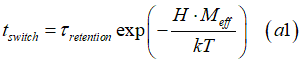
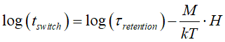
The Néel model calculates the magnetization switching time tswitch as
where the magnetization Meff is the magnetization of the nucleation domain (case of multi-domain switching) or the total magnetization of the nanomagnet(case of single-domain switching)
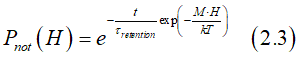
The retention time τretention is the magnetization switching time, when the magnetic field is not applied H=0.
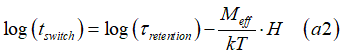
From Eq.(a2) all parameters of thermally-activated switching can be evaluated
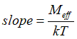
Two. the Néel model is relatively simple and only has two free parameters: the energy barrier Ebarrier and the rate of interaction finter of the nanomagnet with the magnetization-reversing particles (photon, magnon). Alterternatively, any other pair of free parameters may be used (for example, the coercive field Hc and retention time τretention or Meff may be used as one of the two free parameters). However,there are only two independent parameters of the thermally-activated magnetization switching. Additionally, there are parameters, which are related to the magneto-static properties of a nanomagnet. For example, the parameter Δ is proportional to the anisotropy field Hanis and the volume of the nucleation domain is proportional to the magnetization M of the nanomagnet.
(merit 1)![]() (it is the most direct measurement)
(it is the most direct measurement)
It is because the magnetization switching time is the primary parameter of the Neel model of the magnetization switching
(merit 2)![]() (it is free of a possible systematic error)
(it is free of a possible systematic error)
Since it is the direct measurement and the measured dependence in Fig.10 is always linear, a possible systematic error is always clear and can be avoided. See here for details of the systematic errors of other used measurement methods.
(merit 3)![]() (high measurement precision)
(high measurement precision)
The measurement precision of the described method substantially better than the precision of other used measurement methods. The required precision can be reached with a smaller of statistical measurements.
Measurement of Coercive field Hc |
|||||||||
|
|||||||||
| click on image to enlarge it |
(old,incomplete):![]() The magnetic field, at which magnetization is switched between its two stable magnetization directions is called the coercive field
The magnetic field, at which magnetization is switched between its two stable magnetization directions is called the coercive field
(correct):![]() The coercive field is defined as the magnetic field, at which the average magnetization switching time is equal to 1 second.
The coercive field is defined as the magnetic field, at which the average magnetization switching time is equal to 1 second.
![]() High-precision measurement of Hc
High-precision measurement of Hc
The measured dependence of log(tswitch/1 sec) vs H is a line. The coercive field Hc corresponds to magnetic field, at which tswitch=1 sec or log(tswitch/1 sec)=0. A linear fitting experimental data gives the Hc with a very high precision.
(reason 1) Each repeated measurement dives a slightly different value of Hc (See Fig.8)
(reason 2) A measurement at scanning rate of the magnetic field gives different value Hc(See Fig.9)
Yes, this statement is fully correct. However, we can can guess the approximate measurement time of these old measurements. I guess for magnetometer measurement or Hall measurements it may be between 1 and 10 seconds. Therefore, these data can be considered as a rough estimate.
Yes, it is the case of a magnetically soft nanomagnet, in which τretention<1 second (See telegraphic noise below)
Measurement of retention time τretention |
|||||||||
|
|||||||||
| click on image to enlarge it |
![]() The retention time is defined as the average time, after which the magnetization is reversed in the absence of a magnetic field due to a thermal fluctuation.
The retention time is defined as the average time, after which the magnetization is reversed in the absence of a magnetic field due to a thermal fluctuation.
![]() τretention is referred to the maximum data storage time of a magnetic memory.
τretention is referred to the maximum data storage time of a magnetic memory.
![]() Using the described method, the τretention can be measured in the range from one minute to billions of years. The measurement precision is very high (~0.01 %)
Using the described method, the τretention can be measured in the range from one minute to billions of years. The measurement precision is very high (~0.01 %)
Experimentally, the magnetization reversal time tswitch is measured under external magnetic field. In my experimental setup I can measure tswitch in the range from 0.3 s to a few minutes. I adjust the external magnetic field for to be in this range. Since tswitch increases exponentially when H decreases, the tswitch can easily reach a million or billion years when extrapolated to H=0. It depends of the slope of Fig.10 and Hc
![]() High-precision measurement of τretention
High-precision measurement of τretention
The measured dependence of log(tswitch/1 sec) vs H is a line. The retention time τretention corresponds to the magnetization switching time, when the magnetic field is not applied H=0. A linear fitting experimental data and extrapolating the line to H=0 give the τretention with a very high precision.
The Néel model calculates the magnetization switching time tswitch as
Eq.(a1) can be re written in a linear form as
The linear fitting the experimental data of Fig.10, Fig.12, Fig.13 gives the τretention with a very high precision.
Measurement of the size of nucleation domain |
||||||
|
||||||
| Measurement of the size of nucleation domain consists of two measurements: (switching measurement): slope of log( tswitch ). (magnetostatic measurement) magnetization of ferromagnetic metal of nanomagnet | ||||||
| click on image to enlarge it |
![]() (What one needs to measure the domain size): magnetization of the sample + the slope of the log of the switching probability. Substution of the data into Eq.(a4) below gives the volume of the nucleation domain
(What one needs to measure the domain size): magnetization of the sample + the slope of the log of the switching probability. Substution of the data into Eq.(a4) below gives the volume of the nucleation domain
 (a simple idea beyond measurement: ) The log of switching probability is proportional to the number of the spins in the nucleation domain, which is a product of the volume of the nanomagnet and the number of spins per volume (= magnetization of the ferromagnetic material). The external magnetic field changes the magnetic energy of each spin and, correspondingly, the switching probability. Consequently, the change of log of probability under the external magnetic field is linearly proportional to the number of the spins in the nucleation domain and, therefore, the volume of the nucleation domain.
 When the dimensions of a nanomagnet are sufficiently small, the magnetization reversal occurs in a single domain. It means that the magnetization at all points of the nanomagnet rotates coherently and the magnetization in different parts of the nanomagnet remains parallel during the rotation. When the dimensions of the nanomagnet become larger, the type of the magnetization reversal is changed to the multi-domain type In the case of a larger nanomagnet, it is more energetically favorable when at first the magnetization of only a small domain is reversed following by domain wall movement expending the region of the reversed magnetization over the whole nanomagnet.
 Simple math beyond measurement of the domain size
If the probability to reverse the spin of one electron equals p, then the probability to reverse the spin of two electrons equals p·p. The probability to reverse the spin of n- electrons equals pn. The magnetization M of a ferromagnet is defined as a number of the spins per the ferromagnet volume. If the volume of the ferromagnetic domain is Vdomain , the number of the spin in the domain is M ·Vdomain. Then, the probability of a reversal of the nucleation domain is calculated as
pdomain=pM ·V_domain
or log(pdomain) =M·Vdomain
The switching probability of one spin is larger for a longer waiting time and proportional to the energy barrier Ebarrier (classical model) or the Zeeman energy EZeeman (quantum model)
tswitch~eE/kT
The magnetic energy of the spin in an external magnetic field H equals to
E=H·μ=H·g·μB·S
The log switching time for one spin is
log(tswitch)~ H·g·μB·S
The switching time of the n electrons depends on the external magnetic field as
log(tswitch)~ H·g·μB·S·n=H·slope,
where g is the g-factor and μB is the Bohr magneton
Therefore, the slope is linearly proportional to the number of the spins in the nucleation domain.
![]() The slope of Fig.13 gives the magnetization of the nucleation domain. From the known (measured) magnetization of the ferromagnetic metal per its volume , the volume of nanomagnet is calculated
The slope of Fig.13 gives the magnetization of the nucleation domain. From the known (measured) magnetization of the ferromagnetic metal per its volume , the volume of nanomagnet is calculated
The log magnetization switching time log (tswitch ) is linearly proportional to the external magnetic field (See here):
![]()
where the slope of this dependence is calculated as
the magnetization Meff is the magnetization of the nucleation domain (case of multi-domain switching) or the total magnetization of the nanomagnet(case of single-domain switching)
Magnetization of the ferromagnetic metal of the nanomagnet Mmagnet per volume Vmagnet of can be measured by a magnetometer (or checked by literature).
Since the magnetization of the nucleation domain is measured, the volume of the nucleation domain is calculated as
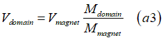
in conventional units the nanomagnet volume is calculated as
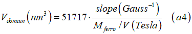
the number 51717 is a product of the fundamental constants (see above) in the shown units.
(note) The magnetization, which is measured by a magnetometer, is a sum of the total spin of the localized electrons and the total spin of the conduction electrons. In Eq.(a4), only the total spin of the localized electrons should be used. However, the precise measurement of the total spin of the spin-polarized conduction electron is still challenging (See here). The use of the measured magnetization in Eq.(a4) gives a good estimate of Vdomain, which is slightly smaller than the real value of Vdomain.
Hysteresis loop of a nanomagnet |
||||||||
|
||||||||
| Different magnetization switching mechanisms in a nanomagnet with and without static domains is the reason of different shape of the hysteresis loop. | ||||||||
| Click on image to enlarge it |
It is the feature of a nanomagnet or a magnetic film of a larger area. The static magnetic domains usually exists in the absence of the external field. However, sometimes some external magnetic field is required in order to the static magnetic domain. The static magnetic domains are formed to make a balance between the exchange force, which is trying to align all magnetization of all regions to be in one direction, and magnetitic dipole force, which is try to align the magnetization in neighbor regions to be antiparallel.
Note: The FeB and FeCoB nanomagnets of size of a few micrometers and smaller do not have any static domains. The magnetization of the whole nanomagnet is in one direction.
Note: A nanomagnet free of static magnetic domains have a rectangular- shape hysteresis loop (See Fig.1). The hysteresis loop of a nanomagnet with static domains is not rectangular shape. It is either of shape shown in Fig.2 or with some steps.
Magnetization switching mechanism of a nanomagnet with static domains: domain wall expansion of static magnetic domains.
The switching domain exists in a moderate-size nanomagnet, which are free of static domains. When an external magnetic field is applied opposite to the magnetization direction. At first, the magnetization of a small region (of the switching domain) rotates to be parallel to the external magnetic field. Next, its domain wall of the switching domain expands over the whole nanomagnet. The life time of the switching domain is short ( less than o millisecond).
Note: The size of the switching domain in FeB and FeCoB nanomagnets is varied from 30 nm to 90 nm depending on the material and structural defects in the nanomagnet. The size of the switching domain in nanomagnet of reasonably-good quality is 45-55 nm.
Measurement of parameter Δ |
||||||
|
||||||
| high-precision measurement of the Δ consists of two measurements: (switching measurement): slope of log( tswitch ). (magnetostatic measurement) anisotropy field Hanis | ||||||
| click on image to enlarge it |
The parameter Δ describes the energy required for the magnetization reversal in comparison with thermal energy. The parameter Δ is defined is the ration the energy barrier to the thermal energy
Δ = Ebarrier/kT
The parameter Δ is a parameter, which estimates the ability of a memory cell to withstand a thermal fluctuation and the ability to withstand the temperature rise without loss of the stored data. It is defined as the ratio of energy barrier Ebarrier in the absence of an external magnetic field to the thermal energy kT.
In the case of multi-domain switching, the magnetic energy is the energy of the nucleation domain.
In the case of single-domain switching, the magnetic energy is the energy of the whole nanomagnet.
The magnetic energy or the PMA energy can be calculated as (See PMA)
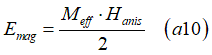
where Meff is the magnetization of the nucleation domain (case of multi-domain switching) or .the total magnetization of the nanomagnet(case of single-domain switching) and Hanis is the anisotropy field. The Hanis is the feature of the PMA and the same for the whole nanomagnet and the nucleation domain. From Eq.(a10) the parameter Δ can be calculated as
![]()
The retention time can be calculated from Δ as
Transformation of Hysteresis loop |
||||||||||||
|
||||||||||||
| The x-axis is applied out-plane magnetic field. Click on image to enlarge it. |
Switching time influenced by different effects |
||||||||||||||||||||
|
||||||||||||||||||||
| Click on image to enlarge it. |
Results of Néel model |
| (main result): magnetization switching time tswitch vs magnetic field H |
|---|
 |
 |
| logarithm of the magnetization switching time log( tswitch ) vs H is linearly proportional to external magnetic field H. The proportionality coefficient is the magnetization M of a nucleation domain for switching (multi-domain switching) or the magnetization M of nanomagnet (single-domain switching) |
| (result 2): Energy barrier Ebarrier between two stable states of a nanomagnet is linearly proportional to external magnetic field H |
| Click on image to enlarge it |
Assumption of the the Néel model. The Néel model assumes that the switching between two stable magnetization states occurs when the energy of a thermal fluctuation becomes larger the energy barrier Ebarrier between states. The probability of a thermal-fluctuation is described by the Boltzmann distribution
(Ignored Fact 1) ![]() Spin conservation law
Spin conservation law ![]()
The spin conservation law requires the participation of a particle with a non-zero spin (a magnon, photon etc) in the magnetization reversal process. The Néel model assumes that particles participate in the magnetization reversal, but only particle energy is used in the calculation of the Néel model.
(Ignored Fact 2) ![]() Complex dynamic of magnetization reversal
Complex dynamic of magnetization reversal ![]()
The complex dynamics of the magnetization reversal should be described by the Landau-Lifshitz (LL) equations, and a model of the thermally-activated magnetization reversal should be based on the LL equation. This dynamic is fully ignored the Néel model. The dynamic of the magnetization reversal is only important for the resonance switching. The Brown- is one possible model, which describes the resonance switching (See here)
(Ignored Fact 3) ![]() Dynamic of movement of domain wall
Dynamic of movement of domain wall![]()
It assumed that after a nucleation domain for the magnetization reversal is created, it has a sufficient energy to move without any pinning over the whole nanomagnet.
(step 1) Calculation of the energy barrier Ebarrier
(step 2) Calculation of the switching probability
(step 3) Calculation of the magnetization switching time
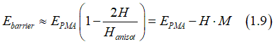
The angle-dependent part of the energy E of the uniaxial magnetic anisotropy can be written as
![]()
where θ is the angle between the magnetization M and the film normal, φ is is the angle between the magnetic field H and the film normal, EPMA is the energy of the perpendicular magnetic anisotropy, which includes the energy due to the demagnetization field.
Below the case when a magnetic field is applied along the magnetic easy axis (perpendicularly to the film) ( φ=0) is calculated. The maximums of energies can be found from the condition
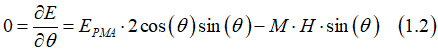
Maximum of energy is at θ max
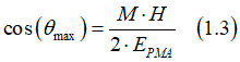
with corresponded energy of

Maximum of energy is at θ min=0 and 180 degrees
|
||||||||||||
|
||||||||||||
|
||||||||||||
| click on image to enlarge it |
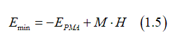
Therefore, the barrier height is
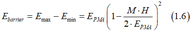
The PMA energy Ebarrier can be express as
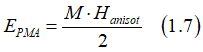
where Ebarrier is the anisotropy field (See here). Substituting Eq. (1.7) into Eq.(1.6) gives
magnetization-reversal time τ vs magnetic field (Eq.(1.15)) |
||||
|
||||
|
||||
| The crossing of the line with the y-axis gives retention time τretention | ||||
The crossing of the line with the x-axis gives coercive field Hc |
||||
| The slope of the line is proportional to the Meff (magnetization of a nucleation domain for switching (multi-domain switching) or magnetization of nanomagnet (single-domain switching)) | ||||
| Data measured: jan. 2018. Click on image to enlarge it |
In all my measurements of magnetic nanomagnet it always the coercive field Hc is about 2-4 % of the anisotropy field Hanisotrp. Therefore, Hc / Hanisotrp ~ 0.02-0.04 at measurement time of 1 s.
As was aforementioned, the switching field becomes larger as the switching time becomes shorter. In my experimental setup, the shortest measurement time is 100 ms and the condition Hc << Hanisotropy is well satisfied. However, in the case of a shorter measurement time, the condition may be not satisfied. The extension of the reported results for that case is straightforward.
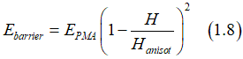
Using this assumption, the Eq.(1.8) is simplified as
or
![]()
where M is the magnetization of a nucleation domain for switching (multi-domain switching) or the magnetization of nanomagnet (single-domain switching))
It is means that the measurements of the thermally- activated switching is done at a moderate or a small magnetic field. In the case of a high magnetic field H ~ Hanisotropy , the magnetization switching is very rapid. The magnetization is switched within time of a nanosecond or shorter. It means that the magnetization turns along the external magnetic field almost instantly after it applied. It is not practical to make a measurement for such high field and a short switching time. The practically-measurable switching time of a millisecond or a second or a minute is for a small or moderate magnetic field when H << Hanisotropy. The Hc is defined as the field when the average switching time is one second.
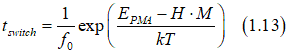
Néel model states that the average magnetization reversal time tswitch or relaxation time τ is described by the Arrhenius low:
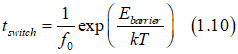
where f0 is is the so-called attempt frequency associated with the frequency of the gyromagnetic precession; Ebarrier is the energy barrier between two states when the magnetization is along and opposite to the external magnetic field.
![]() The Arrhenius low has its origins in the 1880s when Arrhenius proposed, from an analysis of experimental data, that the rate coefficient in a chemical reaction should obey the law
The Arrhenius low has its origins in the 1880s when Arrhenius proposed, from an analysis of experimental data, that the rate coefficient in a chemical reaction should obey the law
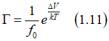
where ΔV denotes the threshold energy for activation of the chemical reaction, f0 is the attempting frequency.
Main result of Néel model |
|
|
| logarithm of the magnetization switching time log( tswitch ) vs H is linearly proportional to external magnetic field H. The proportionality coefficient is the magnetization M of a nucleation domain for switching (multi-domain switching) or the magnetization M of nanomagnet (single-domain switching) |
|---|
| Click on image to enlarge it |
Substituting Eq. (1.8) into Eq.(1.11) gives
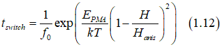
In the case when Hc << Hanisotrp , Eq(1.12) is simplified to
the retention time τretention is the average time of magnetization reversal without any external magnetic field. From Eq.(1.13), the τretention can be calculated as
From Eqs.(1.13 and 1.14) , the magnetization reversal time τ is given as:
![]()
The linear dependence of log( tswitch ) vs H perfectly fit to all experimental measurements. It clearly proves that the classical Néel model fully describes the non-resonance magnetization reversal.
(result of the Néel model):![]() The logarithm of the magnetization switching time log( tswitch ) vs H is linearly proportional to external magnetic field H. The proportionality coefficient is the magnetization M of a nucleation domain for switching (multi-domain switching) or the magnetization M of nanomagnet (single-domain switching)
The logarithm of the magnetization switching time log( tswitch ) vs H is linearly proportional to external magnetic field H. The proportionality coefficient is the magnetization M of a nucleation domain for switching (multi-domain switching) or the magnetization M of nanomagnet (single-domain switching)
Alternative method to measure Hc and Δ |
||||||
|
||||||
| this methods are not recommended, because the probability of a systematic error for these methods is very high | ||||||
| Click on image to enlarge it |
The probability of a systematic error for each of below-described methods is very high. The convergence of some of this methods is not fast.
Alternative methods to measure Hc and Δ :
(method 1): graded magnetic field
(method 2): graded pulsed magnetic field
(common error 1) ![]() unjustifiably large number of free parameters is used to fit experimental data.
unjustifiably large number of free parameters is used to fit experimental data.
The Néel model is relatively simple and only has two free parameters: the energy barrier Ebarrier and the rate of interaction finter of the nanomagnet with the particles (See details of the Néel model). Alterternatively, any other pair of free parameters may be used (for example, the coercive field Hc and retention time τretention or size of nucleation domain may be used as one of the two free parameters). However, maximum two parameters should be always used for the data fitting. Additionally, there are parameters, which are related to the magneto-static properties of a nanomagnet. For example, the Δ is proportional to the anisotropy field Hanis (See Eq.(a7)) and the volume of the nucleation domain is proportional to the magnetization M of the nanomagnet (See Eq.(a3)). Both Hanis and M can be measured from an independent magneto-static experiment without the use of any thermally-activated switching measurements. The magnetization M of a ferromagnetic metal can be measured by a magnetometer. Hanis can be measured by applying an in-plane magnetic field and monitoring the in-plane component of the magnetization (See here).
The fact that there are only two free parameters of the Néel model, can be confirmed from measured dependence of tswitch on H (See here). A straight line perfectly fits to all experimental data and the line is described by only two free parameters.
(common error 2) ![]() Assumption that the attempt frequency f is a universal constant of the Néel model and equals to 1 GHz
Assumption that the attempt frequency f is a universal constant of the Néel model and equals to 1 GHz
It is hard to trace from which reason this assumption came from, but it is completely incorrect assumption (See details of the Néel model).
(common error 3) ![]() Incorrect use of statistical measurement and statistical analysis.
Incorrect use of statistical measurement and statistical analysis.
![]() Example: A common systematic error of measurement method of graded pulsed magnetic field (See here)
Example: A common systematic error of measurement method of graded pulsed magnetic field (See here)
The Néel model assumes that the magnetization reversal occurs only when the spin of the nanomagnet interacts with a "non-zero-spin" particle (a magnon, a photon etc.), which energy is higher than the barrier height Ebarrier between two stable states of the nanomagnet. The temperature is assumed to be sufficiently high so that the energy distribution of the particles is described by the Boltzmann distribution. Therefore, the number of particles, which are able to reverse the magnetization, is calculated from the the Boltzmann distribution as
where n0 is the total number of the particles, which are able to reverse the magnetization(e.g. the total number of magnons,phots,etc.). When there are more particles, the probability of reversal becomes higher. The frequency, at which the magnetization can be reversed, is proportional to the number of the particles and is calculated as
where finter is the frequency of interaction of one particle with the spin of the nanomagnet.
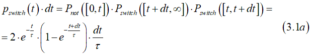
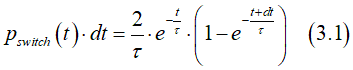
The probability Prever(t,t+dt) of the magnetization reversal in a small time interval between t and t+dt is calculated as
![]()
where 
The probability Pnot(t,t+dt), that the magnetization is not reversed during the time interval dt, is calculated is
![]()
If the magnetization is not reversed in the interval [t0,t+dt], that means that it is not reversed in both intervals [t0,t] and [t,t+dt]. Therefore, the probability Pnot(t0 ,t+dt) is calculated as
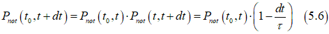
Eq.(5.6) can be simplified as
![]()
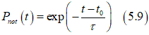
The function Pnot(t) is defined as the probability of non-reversal of the magnetization in the time interval from t0 to t. From Eq. (5.7), the function Pnot(t) satisfies the following differential equation:
![]()
In the case when the external magnetic field H is a constant and time-independent, the energy barrier Ebarrier and τ are time-independent as well and Eq. (5.8) becomes a linear differential equation. The solution of Eq.(5.8) gives the probability Pnot(t) of the non-reversal of the magnetization in the time interval from t0 to t as:
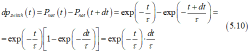
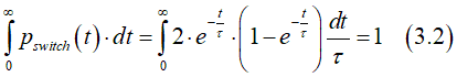
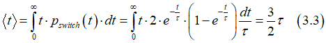
Next, the averaging magnetization switching time tswitch is calculated. If the external magnetic field is switched on at time t0=0 in the direction opposite to the magnetization, the probability dpswitch that the magnetization is reversed in the time interval between t and t+dt is the difference between probabilities that it is not reversed until time t and until time t+dt:
From Eq. (5.10), the averaging magnetization switching time tswitch is calculated as
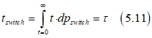
The substitution of Eq.(5.4) into (5.11) gives the Arrhenius law (Eq.(1.10)) as
![]()
pulse magnetic field to measure tswitch |
||||
|
||||
This measurement should be used in case when a time of measurement of magnetization direction is comparable with tswitch (e.g. Hall measurement) |
||||
| Data measured: jan. 2018. Click on image to enlarge it |
Note 1 (measurement of magnetization reversal event) ![]() An event of magnetization reversal is monitored by a measurement of a material parameter, which depends on the magnetization oft he nanomagnet (e.g. resistance, tunneling resistance, magneto-optical constants, Hall angle etc.)
An event of magnetization reversal is monitored by a measurement of a material parameter, which depends on the magnetization oft he nanomagnet (e.g. resistance, tunneling resistance, magneto-optical constants, Hall angle etc.)
Note 2 (long time for measurement of Hall voltage) ![]() The Hall voltage is small and can be measured by a nanovoltmeter. One measurement by a nanovoltmeter takes 1.7 second
The Hall voltage is small and can be measured by a nanovoltmeter. One measurement by a nanovoltmeter takes 1.7 second
In order to measure tswitch shorter than 5 second using the Hall setup, the pulsed magnetic field should be used.
In order to measure tswitch longer than 5 second the use of the pulsed magnetic field is not necessary.
It is a ration of the magnetization switching events to the sum of switching and non-switching events for a fixed measurement time. The switching probability can be measured experimentally.
The probability that the magnetization is not switched by the time t is described as
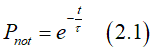
where τ is the relaxation time
Correspondingly, the probability that the magnetization is not switched by the time t is described as
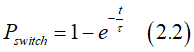
In the case when H<< Hanisotrp, substituting Eq(1.15) into Eqns.(2.1-2.2) gives
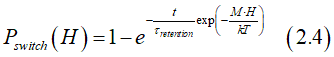
It is easier and simpler to calculate the probability of not switching Pnot by time t rather than the probability of switching Pswitch by time t. The relation between Pnot and Pswitch is straightforward Pnot + Pswitch=1
The non- switching of the magnetization in time interval interval [0,t+dt] means that the magnetization is not switched in both time intervals [0,t+dt] and [t,t+dt]. The probability of non-switching in time interval [0,t+dt] equals to the product of probabilities of non-switching in time intervals [0,t+dt] and [t,t+dt]:
![]()
Probabilities of switching in a small time interval [t,t+dt] is linearly proportional to dt
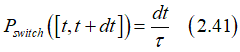
where 1/τ is the coefficient of the proportionality.
From Eq.(2.41) we have
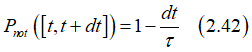
Substituting Eq.(2.42) into Eq.(2.40) gives
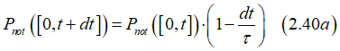
From time t to t+dt the value of the non-switching probability change on
![]()
Substituting Eq.(2.40a) into Eq.(2.43) gives
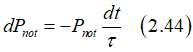
Case 1. External magnetic field is constant
in this τ is constant. The integration of Eq.(2.44) gives
Case 2. External applied magnetic field changes in time
Substituting Eq.(1.8) into Eq.(2.47) gives

where
Case 3. External magnetic field linearly ramped in time
For example, if time dependence of magnetic field is described as
Using integral
and substituting Eq.(2.6) into Eq.(2.48) and integrating gives
Case 4. External applied magnetic field linearly ramped in time and it is H(t)<<Hanisotropy (realistic case)
In the case of small field H(t)<<Hanisotropy, the following approximation can be used
substituting Eq(2.49a) into (2.48) gives
In the case of linear ramping
integration of (2.49c) gives

where 
Meff is the effective magnetization or the magnetization of a nucleation domain
![]()
Case when External magnetic field linearly ramped
In this case time dependence of magnetic field is described as
below I calculate as switching probability depends on the measurement time ( duration of magnetic pulse).
Probability that magnetization is switched only in time interval between t and t+dt is equal to the product of probability that it is not switched
where switch probability exactly at time t will be
The probability was normalized so that
The average magnetization-reversal time is calculated as
Alternative measurements of Hc. Rough measure of switching field |
||||||
|
||||||
This measurement gives coercive field Hc |
||||||
| Data measured: jan. 2018. Sample:200-nm wide 25-um long Ta(8)/FeB(0.9)/MgO(7.1)/Ta(1)/Ru(5) nanowire. Number of measurements is 80. Two distributions, which is obtained from a direct fit by Eq.(4.4) or from average switching field Eq.(4.8), are shown. Click on image to enlarge it |
Below I calculate the dependence of the switching probability on magnetic field.
Below only the realistic case of H<< Hanisotrp is calculated. The switching probability in this case is described by Eqs. (2.3),(2.4)
As was show above, the coercive field (switching field) depends on the measurement time τ (see Fig.11). Let us refer to the coercive field as the switching field at measurement time of 1 second τ=1. Than, from Eq.(1.15)
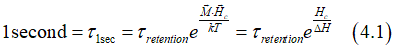
Using Eq.(4.1), Eq.(1.15) is simplified to
![]()
Substituting Eq.(4.3) into Eqs.(2.1) and (2.2) gives the probability Pnon-switch([0,H]), that the magnetization is not switched, when magnetic field increases from o to H, and the probability Pswitch([0,H)), that the magnetization is switched, as
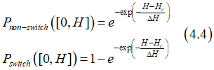
The probability Pswitch([H,H+dH)) that the magnetization is switched at the magnetic field between H and H+dH is proportional to
![]()

where A is the proportionality constant, which can from normalization condition
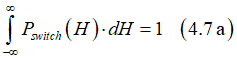
and it gives the switching probabilities as
The average switching magnetic field is calculated as
![]()
The mean deviation is calculated as
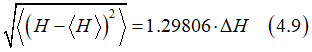
In normalization
the following integral was used
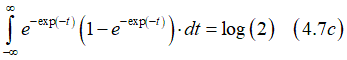
to obtain the distribution
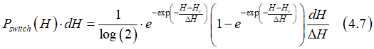
The average field is defined as
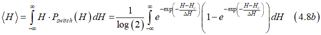
Substituting Eq.(4.7) gives
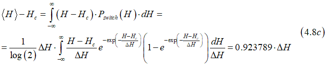
We used the value of the integral
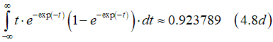
Eq(4.8c) gives
![]()
The mean deviation is defines as
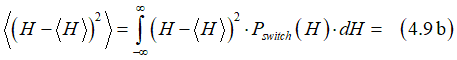
Substituting Eqs. (4.7) and (4.8) gives
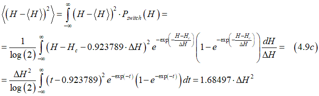
or
Fig.15. Measurement of anisotropy field Hanisotropy |
||
|
||
| The arrow shows the direction and magnitude of the applied in-plane magnetic field. The ball shows the magnetization direction. Without magnetic field the magnetization is perpendicularly-to-plane. Under magnetic field, the magnetization turns toward magnetic field. The field, at which the magnetization turns completely in-plane, is called the anisotropy field. The dots of the right graph shows experimental data. Measurement date: May 2018. | ||
| Click on image to enlarge it |
According to Neel model, the energy barrier Ebarrier between two stable magnetization states in absence of magnetic field equals to EPMA. Therefore
The retention time can be calculated as
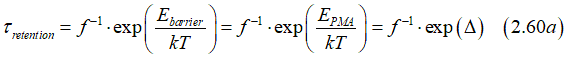
or
![]()
There are three possible techniques to measure Δ. Each technique requires additional measurement of Hanisotropy (see here the measurement details).
The Δ is evaluated by fitting the distribution of magnetization switching probability Eq.(2. 49b) or (2.8).
The Δ is evaluated from the width of the distribution of magnetization switching probabilities Eq.(4.2) and Eq.(4.7).(See Fig.12)
The Δ is evaluated by from measurements of the dependence magnetization-reversal time vs magnetic field(See here )
This high-precision measurement of Δ requires 3 steps
step 1 : Measuring the effective magnetization Meff
On log scale, τ is linearly proportional to the applied magnetic field(Fig.11). The slope of the fitting lines is proportional to Meff and the horizontal offset is proportional to τretention
step 2 : Measuring the anisotropy field Hanisotropy
Method to measure anisotropy field is described here
It is a relatively easy to measure the anisotropy field (See here) . Even though it often requires a relatively large in-plane magnetic field. Without magnetic field the magnetization is perpendicularly-to-plane. Under magnetic field, the magnetization turns toward magnetic field. The field, at which the magnetization turns completely in-plane, is called the anisotropy field. The EPMA is calculated from Hanisotropy as (See here)
where Meff is the total magnetization in the case of a single-domain magnetization reversal or the effective magnetization Meff in the case of multi-domain magnetization reversal
step 3 : Calculating Δ
The Δ can be simply calculated as:
Any method related to Neel model is based on only one important parameter, which is the barrier height Ebarrier between two stable magnetic states:
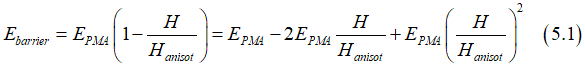
There are three component, which are proportional to magnetic field H in power 0, 1,2.
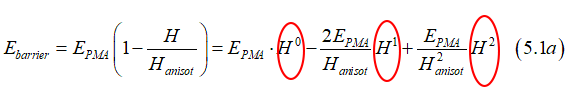
The Δ can evaluated from independent measurements of the 2d and 3d components.
Effective magnetization Meff. Magnetization reversal in a ferromagnetic nanowire |
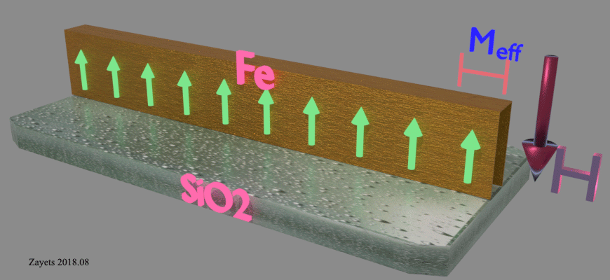 |
| When a magnetic field is applied opposite to the magnetization direction,at first the domain wall (blue line) is formed. Within this domain the magnetization is reversed by a thermal activation (Neel mechanism). Next, the domain wall moves along the nanowire. When it stops, only a small domain remains. Its magnetization is reversed by a thermal-activation as well. |
| Click on image to enlarge it |
Multi- domain magnetization switching
When size of the nanomagnet is sufficiently large, the magnetization reversal is not coherent over whole nanomagnet. At first, the magnetization is reversed in a small domain. Next the domain wall moves and expands. As a result, the magnetization of whole nanomagnet becomes along the applied external magnetic film.
The Meff is magnetization of first magnetic domain, which triggers the magnetization reversal.
![]() The reason, why magnetization switching occurs by this mechanism:
The reason, why magnetization switching occurs by this mechanism:
A thermal activation energy to reverse magnetization of a small domain is much smaller, than the energy to reverse magnetization of the whole film.
![]() How small is the size of the nucleation domain
How small is the size of the nucleation domain
The size of the nucleation domain is determined by trade of between the exchange energy and the barrier energy Ebarrier for the magnetization switching. The stronger exchange interaction is, the larger size of the nucleation domain become.
The size of the nucleation domain is evaluated from measurements of Fig.11
Single-domain magnetization switching
In this case the magnetization of whole nanomagnet is reversed coherently.
This switching occurs only in a nanomagnet of very small size (diameter ~10-40 nm)
Meff equals to the saturation magnetization Msat of material multiplied by the sized of the nanomagnet
Meff gives the magnetization of the initial domain, which is first switching during magnetization (case of multi-domain switching). In the case of single-domain reversal, Meff equals to product of the saturation magnetization and the volume of nanomagnet.
This method can unambiguously measure for a tested device whether magnetization switching is single-domain or multi-domain.
single-domain switching
It is the case when the effective magnetization Meff is equal to the saturation magnetization M multiply to volume of the nanomagnet
multi-domain switching
It is the case when the effective magnetization Meff is smaller than the saturation magnetization M multiply to volume of the nanomagnet
|
||||||
| Samples of different width and length are shown. The widths of FeB nanomagnets are from 100 to 3000 nm. Lengths of nanomagnets is from 100 to 20000 nm. Samples with Ta and W buffer are shown. FeB and FeB multilayers of different thicknesses are shown. | ||||||
| Click on image to enlarge it. Zayets 2018. |
![]() The size of nucleation domain equals the effective magnetization Meff divided per the saturation magnetization M.
The size of nucleation domain equals the effective magnetization Meff divided per the saturation magnetization M.
The saturation magnetization M is measured by SQUID magnetometer before nano fabrication and The the effective magnetization Meff is measured by this method after micro fabrication.
![]() FeB and FeCoB amorphous nanomagnet + anneal and partial recrystallization
FeB and FeCoB amorphous nanomagnet + anneal and partial recrystallization
As can be seen from the right picture, the size of the nucleation domain varies from 30 nm to 60 nm. However, there are nanomagnets with a longer domain size.
The variation is narrow: from 40 nm to 50 nm. H
Influence of interface on effective magnetization Meff |
||||||
|
||||||
| Sample: Ta(5):FeCoB ( 1 nm, x=0.3):MgO(7) Volt58A (L58B); nanowire width is 3000 nm, nanowire length is 25 um, length of etched section is 3 um | ||||||
| Click on image to enlarge it | ||||||
Experiment to test the influence of the interface on magnetic properties of nanowire.
The key feature of this experiment: MgO is removed from a half of nanowire and the magnetic properties of both parts are measured. Since all magnetic properties of both are identical except
Similar slope of lines of right figure indicate that the effective magnetization Meff is nearly the same for both parts. It means that the etching was stopped just after MgO and FeCoB was not etched
Effect of Removal of MgO:
1) Anisotropic field: decreases
2) Magnetization: no change
3) Coercive field decreases
4) Retention time: decreases
5) Effective magnetization : no change
6) Delta: decreases
7) nucleation domain size: no change
8) Hall angle: decreases
| part where | anisotropy field, kG | retention time 10^ s | Meff E24 T m3 | coercive field, Oe | Δ | nucleation domain size, nm | Hall angle, mdeg |
|---|---|---|---|---|---|---|---|
| MgO is not etched | 8.932 | 32.82 | 4.3 | 394.6 | 371.5 | 55.4 | 284.8 |
| MgO is etched | 7.25 | 21.66 | 3.88 | 288.8 | 271.8 | 52.6 | 33.8 |
![]() Note: The Hall angle and Hall resistance in FeCoB nanowire greatly depend on the proximity of MgO gate
Note: The Hall angle and Hall resistance in FeCoB nanowire greatly depend on the proximity of MgO gate
delta Δ vs retention time τretention |
||||
|
||||
| Δ vs retention time τretention (logarithmic scale). Each point corresponds to a different temperature of nanomagnet. When the temperature increases, both the Δ and the retention time τretention decrease. | ||||
| The experimental data proves the validity of Eq.(2.60). | ||||
| Click on image to enlarge it |
Both the delta and retention time characterize the probability of the magnetization switching in absence of a magnetic field.
The relation between them is (See here)
or
![]()
![]() Experimentally the retention time and the Δ are measured by two independent experiments (see here and here)
Experimentally the retention time and the Δ are measured by two independent experiments (see here and here)
 All my experimental data (by Nov. 2018) show that the delta linearly proportional to log of the retention time.
note: Experimental data are better fitted by
![]()
where 0<a<1
All my experimental data (by Nov. 2018) show that attempt frequency f is nearly the same for all samples made of the same ferromagnetic metal. However, it is different for different metals. For example, there is a two order difference between f in samples made of an amorphous FeB and made of a single crystal Co.
temperature dependence of delta Δ |
temperature dependence of Hall Angle |
temperature dependence of anisotropy field |
|---|---|---|
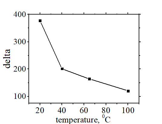 |
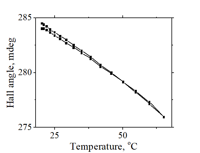 |
 |
| Δ rapidly decreases with increases of temperature. The temperature dependence of EPMA mainly defines temperature dependence of Δ. | Hall angle always decreases with increase of temperature. For temperatures far from Curie T, the decrease is nearly linear. | Hanis rapidly decreases with increases of temperature. It is similar to T dependence of Δ |
| Click on image to enlarge it | Sample: Ta(5):FeCoB ( 1 nm, x=0.3):MgO(7) Volt58A (L58B) | Sample: Volt58A (L58B) |
When temperature rises, all the Hall angle , coercive field, anisotropy field, effective magnetization, saturation magnetization, retention time and nucleation domain size decrease
A. No. The decrease of the Δ with a temperature rise is more sharp. It is because EPMA substantially decreases with a rising of temperature. Additionally, the size of a nucleation domain for magnetization reversal may change with temperature. That also affects the temperature dependance of Δ.
Magnetization switching time for spin-up to down and spin-up to down switching |
Hysteresis loop |
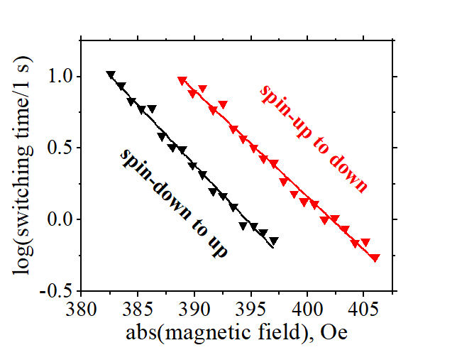 |
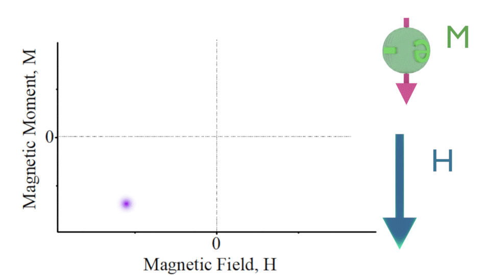 |
| Usually, the lines are parallel with a slight offset. In nanowire with a higher density of defects (domain nucleation centers) the lines may have a slightly different slope and a larger offset | At a negative magnetic field the magnetization is switched from spin-up to spin- down state. At a positive magnetic field the magnetization is switched from spin-down to spin- up state. Click on image to enlarge it |
In principle, the magnetization switching times for switching from spin-up to down state τup-to-down and from spin-down τdown-to-up to up state should be the same
-applying an in-plane magnetic field
- change of temperature
A serious problem of the MRAM is a wide variation of magnetic properties from a cell to cell
The major variation is due to the variation of the domain nucleation size, which may be influence by technology-dependent factors.
In Néel - Brown model, it is assumed that the magnetization switching occurs not because an energy of a thermal fluctuation exceed Ebarrier, but because a more complex magnetization dynamic described by the Landau-Lifshitz equations.
resonance magnetization switching
When frequency of magnetic field, or electrical current or electrical field is close to the frequency of the ferromagnetic resonance (FMR), the magnetization switching may occur at the energy much smaller than the barrier energy Ebarrier.
Example 1: Microwave- assistant magnetic recording (MAMR) to hard disk.
When data density in hard disk becomes very high, the required magnetic field to record one data because unacceptably large. In order to solve this problem the MAMR is used.
In the case of MAMR, a weak microwave radiation, which frequency is close to the FMR of hard-disk media, excites magnetization precession. After that, the magnetic field of recording head reverses the magnetization and records a data bit. The required recording magnetic field is substantially small than in the case without the microwave radiation.
Example 2: Data recording of magnetic random access memory (MRAM) using the VCMA effect
The VCMA effect is weak effect. At present, it is hard to hard to reverse magnetization by the VCMA effect using DC gate voltage. However, when a pulse of interval close to the reverse of the FMR frequency, the magnetization may be reversed even by small- amplitude pulse (Shiota 2012). In this case, the pulse energy is substantially smaller than Ebarrier.
In the Néel - Brown model, the random magnetic field is assumed to act on the magnetization. The magnetization switching conditions are derived from a solution Landau-Lifshitz equations for the magnetization affected by the random magnetic field.
In the model the random magnetic field is a pure mathematical tool. However, the physical meaning of this fields is associated with the interaction of the magnetization with magnons and the electron scattering (sp-d interaction) between localized d- states and states of spin-unpolarized conduction electrons.
As July 2018, all my experimental measurements fit to the Néel model extremely well (See for example here). Even though I have used the magnetic and electrical pulses at a frequency much smaller than the FMR frequency of my studied samples.
The the Néel model is simple and intuitive. The mathematical description of this model is relatively simple. It is based on two simple facts: (1) there is the energy barrier Ebarrier between two stable magnetization states and (2) the energy of a thermal fluctuation should be larger than Ebarrier.
In contrast, the Néel - Brown model is more complex and less intuitive. The Néel - Brown model should be used only in the case when the Néel model clearly fails to describe the experiment.
FARC measurements |
||||||
|
||||||
| figures from |
This measurement method is used to study features of magnetization reversal
Details of The FORC method can be found in the following references
(Numerical Analysis) In this method a complex hysteresis loop of a multiparticle system is analyzed as a sum of a simple hysteresis loops of each individual particles (mostly square- shape loops). This analysis is called Analysis of Preisach Diagrams.
(FORC Measurement) :![]()
![]() Magnetic properties are evaluated from a set of scan of magnetic field with a different partial reversal of magnetization.
Magnetic properties are evaluated from a set of scan of magnetic field with a different partial reversal of magnetization.
"A FORC diagram is calculated from a class of partial hysteresis curves known as first-order reversal curves or FORCs . As shown in Figure la, measurement of a FORC begins by saturating a sample with a large positive applied field. The field is decreased to a reversal field Ha, and the FORC is defined as the magnetization curve that results when the applied field is increased from Ha back to saturation. This measurement procedure is repeated for different values of Ha to obtain a suite of FORCs (Figure l b). The magnetization at the applied field Hb on the FORC with reversal point Ha is denoted by M(Ha, Hi), where Hi, > Ha (Figure la). Data from consecutive measurement points on consecutive reversal curves (Figure l c; see below) are used to determine the FORC distribution, which is defined as the mixed second derivative:
 "
"
Obviously some researcher are using this method and therefore it might be useful. However, as 2004.04 I cannot see any real benefit of this method in my measurements.
![]() If it is not addressed, the FORC measurement has a substantial systematic error. Similarly to the measurement of coercive field from a coercive loop, the FORC measurement substantially depends on the measurement time, the variation of the measurement time from scan to scan creates a systematic error.
If it is not addressed, the FORC measurement has a substantial systematic error. Similarly to the measurement of coercive field from a coercive loop, the FORC measurement substantially depends on the measurement time, the variation of the measurement time from scan to scan creates a systematic error.
It a rare case of the magnetization reversal for nanomagnet of very specific sizes and thickness.
Systematic measurements in FeCoB nanomagnets of a different structure and composition |
|||||||||||||||||||||
|---|---|---|---|---|---|---|---|---|---|---|---|---|---|---|---|---|---|---|---|---|---|
dependence on anisotropy field Hani |
|||||||||||||||||||||
|
|||||||||||||||||||||
dependence on internal magnetic field Hint |
|||||||||||||||||||||
|
|||||||||||||||||||||
| Dots of the same color and shape correspond to nanomagnet fabricated at different places of the same wafer. Stars show multilayer nanomagnets, which contain several ferromagnetic layers. | |||||||||||||||||||||
| click on image to enlarge it |
 Known tricks and methods of fake and highlight research
E.g. tracing the change Hc as function of a gate voltage or bias current or some another parameter of a weak influence on Hc
(Where is the trick?) ![]() Measurement precision of Hc from coercive loop is very poor. Also, the width of the coercive is slightly different for each measurement. the distribution of measured can be large. (See here method 3 measurements) . The distribution is wide specially for smaller sample. The width of the Hc distribution can be as wide as 50 Oe.
Measurement precision of Hc from coercive loop is very poor. Also, the width of the coercive is slightly different for each measurement. the distribution of measured can be large. (See here method 3 measurements) . The distribution is wide specially for smaller sample. The width of the Hc distribution can be as wide as 50 Oe.
Tricks how to generate a dependence on a gate voltage or bias current:
When I have started my research on VCMA and SOT effects, I have been very surprised about a large difference in reported data on the Hc dependence on gate voltage and bias current. Surprisingly, the opposite polarity of the dependence of Hc on gate voltage has been reported for nearly- identical samples.
Only after I have developed a high precision method of Hc measurement, I have understood the trick. For example, a nanomagnet has Hc =400 Oe with distribution width of 60 Oe. It means the measured from a hysteresis loop is in the range between 370 Oe and 430 Oe. E.g. under gate voltage of - 2 V, the Hc increases to 410 Oe. It means that the range of possible Hc becomes from 380 Oe to 440 Oe. Measuring hysteresis loop several times, it possible to pick a loop with Hc=380 at Vgate=-2 V and a loop with Hc=420 at Vgate=0 V and therefore to show the incorrect opposite dependence of Hc on Vgate. This is how it is possible to make from the same experimental data two opposite dependencies when a low precision measurement method is used.
Many "efficient" magnetization switching by the VCMA or SOT effects has been reported by showing a change of the coercive loop and without a measurement of the change of the retention time
(Where is the trick?) ![]() The property of thermally- activated magnetization switching is that the magnetization can be switched between its two opposite stable directions even without any external magnetic field or a gate voltage or current. The average time, within which the magnetization is switched, is called the retention time. The retention time of FeCoB nanomagnets, which I have been studied, varies from a few seconds to billions of years. For example, the retention time of nanomagnets of sample Volt54A is about an hour. The width of the coercive loop significantly depends on the measurement time. For the case of a fast scan of magnetic field (within 1 second), the loop is wide (It case be assigned as a non-switching case). For the case of a slow scan of magnetic field (within 30 min ), there is almost no width of loop (it can be Hc<0.) (It case be assigned as the switching case). However, nothing basically changed.
The property of thermally- activated magnetization switching is that the magnetization can be switched between its two opposite stable directions even without any external magnetic field or a gate voltage or current. The average time, within which the magnetization is switched, is called the retention time. The retention time of FeCoB nanomagnets, which I have been studied, varies from a few seconds to billions of years. For example, the retention time of nanomagnets of sample Volt54A is about an hour. The width of the coercive loop significantly depends on the measurement time. For the case of a fast scan of magnetic field (within 1 second), the loop is wide (It case be assigned as a non-switching case). For the case of a slow scan of magnetic field (within 30 min ), there is almost no width of loop (it can be Hc<0.) (It case be assigned as the switching case). However, nothing basically changed.
My point is that for thermally- activated switching, the only- important parameter if the change of the retention time. E.g. if the retention time is changed from a billion year to 1 millisecond for example, under an gate voltage, it truly means the magnetization switching by the gate voltage. In contrast, a tiny change of the hysteresis loop should not be considered as the magnetization switching.
Many "champion" data have been reported for magnetization switching of a nanomagnet, when a bias magnetic field is applied in-plane (along the hard axis of nanomagnet)
(Where is the trick?) ![]() As it is shown here, the magnetization under bias of in-plane magnetic field is very unstable and the switching can be triggered by a smallest external perturbation. However, this method is useless for a realistic practical applications, because such switching is very unstable, repeatability is poor and the switching conditions are greatly different from a nanomagnet to a nanomagnet even for those fabricated on the same wafer.
As it is shown here, the magnetization under bias of in-plane magnetic field is very unstable and the switching can be triggered by a smallest external perturbation. However, this method is useless for a realistic practical applications, because such switching is very unstable, repeatability is poor and the switching conditions are greatly different from a nanomagnet to a nanomagnet even for those fabricated on the same wafer.
E.g.
(Where is the trick?) ![]() Measurement
Measurement
(nucleation domain and pinning of domain wall)  In general, there is no pinning of the nucleation domain during the magnetization reversal. Most of nano magnets, I have been studied, have a perfect square-shaped hysteresis loop. If there is a pinning, the hysteresis loop has large steps. (A very small number of nanomagnets I have with such strong pinning) It requires some special efforts in order to make a domain, which is pinned at some place in a nano magnet or a nano wire. I have studied rather simple nano magnets of round, elliptic and square shapes. There was no any specially-made domain-nucleation spot. In this case, the domain unpinning mechanism or the speed of the motion of the domain wall has no influence on the parameters of the thermal activated magnetization switching. It is because in this case the magnetic energy, which requires for the magnetization reversal in the region of nucleation domain (energy for the creation of the nucleation domain) is much higher than the energy of the pinning. Therefore, after the nucleation domain is created, the magnetic energy is already high. Since the high energy of domain-wall motion, after creation of the nucleation domain the domain wall is moving fast and generally it cannot be pinned (except if there is a really-strong domain-pinning site)
(difference of Hc between film & nanomagnet) The coercive loops are very different. The coercive field Hc of continuous film is substantially smaller than Hc of a nanomagnet, which is made from this film. It is because of very different thermal energy, which required for switching in each case. In the case of a continuos film, the magnetization reversal is due to expansion of magnetic domains and the moving of the domain wall. The domain expansion is not a thermally- activated mechanism and itself does not have a hysteresis loop. However, there may be obstacles (defects, surface imperfections, etc) in the film for continuos movement of the domain wall. In this case thermal activation is required in order to overcome the obstacle and therefore the hysteresis loop appears. The thermal- activation energy to overcome the domain pinning is usually small and it causes only small Hc. In contrast, in case of a nanomagnet a substantially larger thermal- activation energy is required in order to create a nucleation domain. This is the reason why the Hc is larger for a nanomagnet.
Coercive loop vs number of defects |
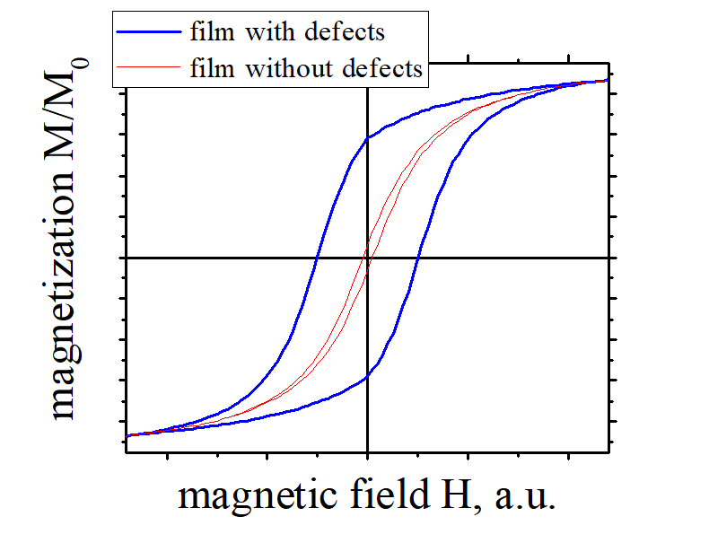 |
| Fig.34 Dependence of coercive loop on number of defects and imperfections in a continuous magnetic film |
| (blue line) is the coercive loop for the film with a large number of defects. The coercive field Hc is large. (red line) is the coercive loop for the same film without defects. There is almost no loop and Hc is almost zero |
| (note) In case of a nanomagnet, the coercive loop is of a rectangular shape. Similarly, the Hc strongly depends on the number of defects and imperfections in the nanomagnet. |
| click on image to enlarge it |
(film quality vs Hc) A measurement of coercive field of continuous film is very useful to estimate the quality of the grown film. The smaller Hc is, the better quality is. The smaller Hc means that there is a smaller number of defects and the average size of defects is smaller. Therefore, it is easier for the domain wall to move.
( Hc of a bulk material without defects) It is correct. A specific coercive field is always associated with bulk ferromagnetic material. For example, Hc~30 Oe for bulk Fe and Hc~200 Oe for bulk Co. Usually the bulk material has an intrinsic fix density of defects, which determines value of . For example, both the bulk Fe and bulk Co are polycrystalline materials. Domain boundary are good pinning sites for domain wall motion, which need a thermal energy to unpin.
An "ideal" ferromagnetic without defects, imperfection or surface roughness doesn't have a coercive loop (Hc =0)
There are many fabrication techniques, which used a dye or a dopant in a ferromagnetic material to pin or unpin a domain wall, in order to make the ferromagnetic material harder or softer
( simulation of hysteresis loop. Case of static domains) There are many rather complex "fancy" methods to simulate the hysteresis loop for the switching by static domain. I use a rather simple, but very effective method. It can be used for a larger sample (not continuous film), in which there are static domains. As the first step, I calculate the loop without the thermally- activated contribution (red line of Fig.34). For this purpose I calculate the size of the static domains as a function of an applied external magnetic field. It can be done by minimizing magnetic energy ( energy of magnetostatic interaction between domains minus energy of domain walls. It can be by Comsol or similar software. At the second step, I measure the parameters of the the thermally- activated switching (This method is major topic of this page. See fig. 10) and include them into the loop. As a result, the red line of Fig 34 transforms into the blue line.
(about stability of magnetic domain vs size of a nanomagnet)
A larger nanomagnets have static domain. The magnetization direction of neighbor domains is usually in opposite directions. It minimizes the energy of the magneto- static interaction between them. When the size of nanomagnet becomes smaller than the size of a magnetic domain, all spins of localized electrons are aligned in one perpendicular direction and the state of the nanomagnet becomes the single-domain state. The reason why all spins of localized electrons are perfectly aligned in a nanomagnet in one direction can be understood as follows. For existence of a static magnetic domain, the positive exchange energy of a domain wall should be balanced by a negative magneto- static energy between dipoles of opposite magnetizations. When shape of nanomagnet is a circle with radius R and domain wall passes through its center, the magneto- static energy is proportional to domain area (~R2) and domain wall energy is proportional to its length (~R). When the size of nanomagnet decreases (decrease of R), the magneto- static energy decreases faster, at some size it becomes unable to balance the domain wall energy and nanomagnet state becomes a single- domain state.
Experimental proof on absence of static domains in a nanomagnet |
 |
Linear dependence of in-plane magnetization vs. in-plane magnetic field. In this measurement, an external magnetic field is applied in plane (along the magnetic hard axis). The magnetization turns towards the in-plane field. The dependence of the in-plane component of the magnetization vs H is a perfect line, which is only possible when the nanomagnet is in a single- domain state. The linear dependence proves that the magnetization turns as whole (as a mono domain) towards the magnetic field instead of a movement of domain wall across nanomagnet as it would be in case of existence of a static domain. |
| click on image to enlarge it |
(reason why magnetization of all regions across a nanomagnet is in the same direction)
In case some region of nanomagnet has the magnetization, which direction is different from the rest of nanomagnet, there is a domain wall of a positive energy between this region and the rest of nanomagnet. The state without this region has a smaller total magnetic energy and is therefore more energetically favorable. For most of nanomagnets, which I have studied, the magnetization is aligned perfectly perpendicularly to surface across the whole nanomagnet.
There are many experimental proofs that the magnetization is perfectly aligned in one direction across the whole. Below there are two which I often use:
(experimental proof 1: linear dependence of M|| vs. H||): In this measurement (details here and here) an external magnetic field H|| is applied in plane (along the magnetic hard axis). The magnetization turns towards the in-plane field. The dependence of the in-plane component of the magnetization M|| vs H is a perfect line, which is only possible when the nanomagnet is in a single- domain state.
(proof of perfect alignment): In the case if some region has magnetization different from the perpendicular, the in-plane magnetic field H|| expands this region in order to minimize the magnetic energy and the dependence is substantially different from linear.
(experimental proof 2: existence of a nucleation domain in process of magnetization reversal ): The experimental measurements of thermally- activated magnetization switching in the same nanomagnets confirms that the magnetization switching mechanism of the studied nanomagnets is the nucleation- domain type. A nucleation domain is an unstable magnetic domain, which exists for a very short time (~a few milliseconds) during magnetization switching. The very existence of the nucleation domain confirms that the sample is mono domain because such nucleation domain can exist only in a single domain nanomagnet in absence of a static domain. Additionally the size of nucleation domain is measured to be between 40 nm and 90 nm for our FeB and FeCoB nanomagnets (details are above). Such measurement is impossible in case when there are static domains.
(proof of perfect alignment): the nucleation domain can exists and therefore be measured in a single- domain nanomagnet. Otherwise, the pre- existed region of different magnetization just expands instead of creation of a nucleation domain.
(experimental proof 3: The stable static domain is at least a few times larger than the unstable nucleation domain. We have exactly similar result (even the measured signal is noisier) for a very small nanomagnets (d<50 nm), which size is even smaller than size of nucleation domain. The existence of a much larger static domain in such a small nanomagnet is absolutely impossible.
(proof of perfect alignment): there is a minimum size of static domain. When the size of nanomagnet is smaller that this size, there is no static domains
(magnetization of a single-domain nanomagnet) When the size of nanomagnet becomes smaller than the size of a magnetic domain, all spins of localized electrons are aligned in one perpendicular direction and the state of the nanomagnet becomes the single-domain state.
The reason why all spins of localized electrons are perfectly aligned in a nanomagnet in one direction can be understood as follows. For existence of a static magnetic domain, the positive exchange energy of a domain wall should be balanced by a negative magneto- static energy between dipoles of opposite magnetizations. When shape of nanomagnet is a circle with radius R and domain wall passes through its center, the magneto- static energy is proportional to domain area (~R2) and domain wall energy is proportional to its length (~R). When the size of nanomagnet decreases (decrease of R), the magneto- static energy decreases faster, at some size it becomes unable to balance the domain wall energy and nanomagnet state becomes a single- domain state.
(about measurement of energy of barrier for domain wall movement) Yes it can be used, but it is very effective.
In fact, the major parameter, which is measured by above - described method, is the energy of the barrier between two stable states of the nanomagnets. The movement of domain wall needs overcomes some energy barriers due to defects and imperfections. The domain overcomes these energy barriers by a thermally- activated mechanism. This reason why the switching by rearrangement of the static domain still has a coercive loop.
If the above - described method is applied for a big nanomagnet with static domain, it measures the average energy of barriers for domain wall movement. Usually, this energy is small and difficult to measure.
![]()
![]() I am strongly against a fake and "highlight" research
I am strongly against a fake and "highlight" research ![]()
![]()
![]()
![]()
![]()
![]()
I will try to answer your questions as soon as possible
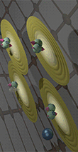
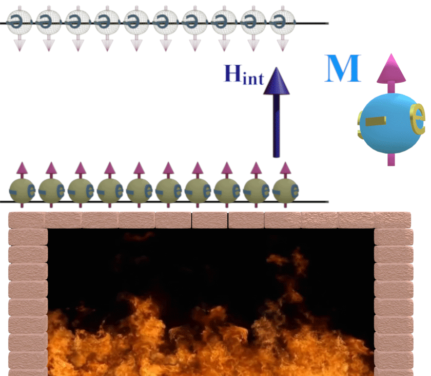
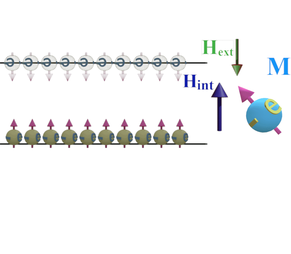
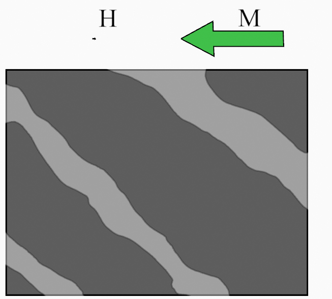
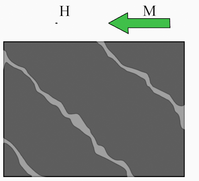
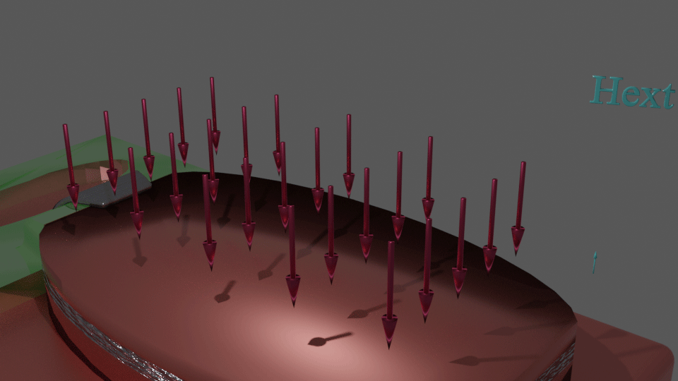
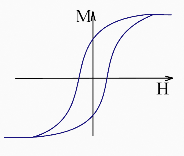
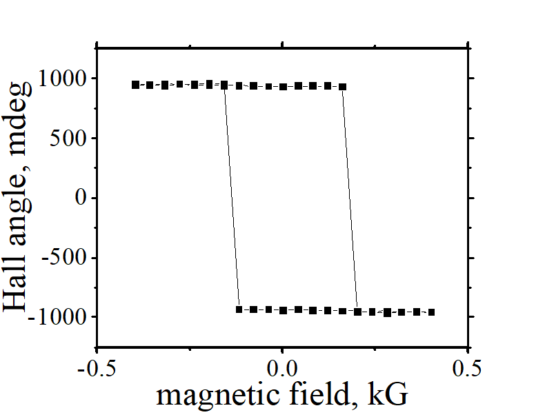
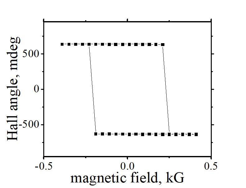
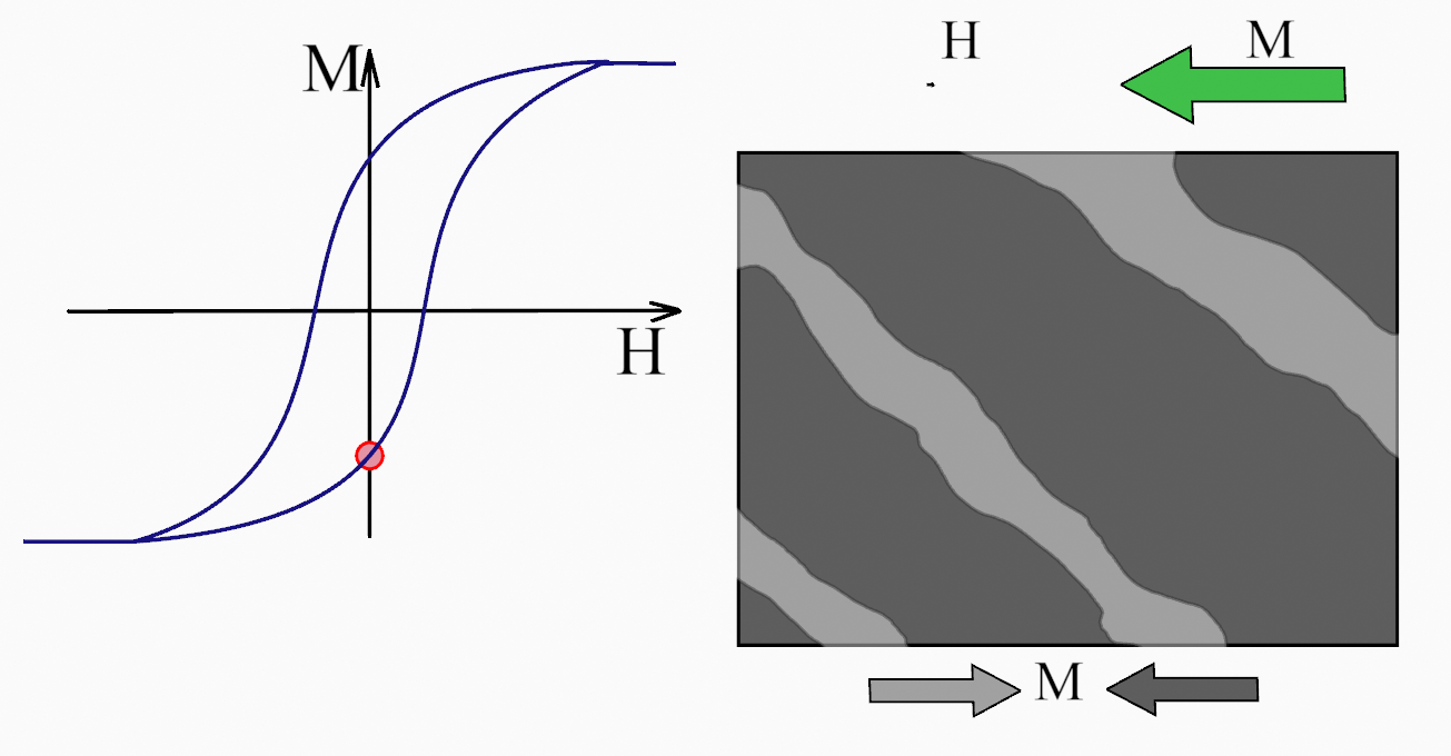
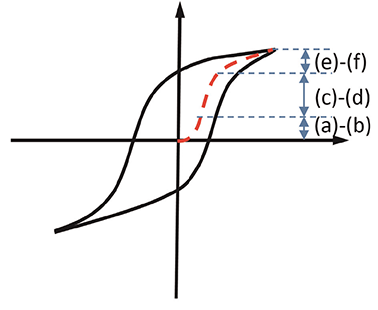
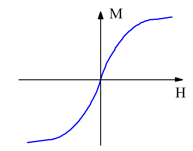
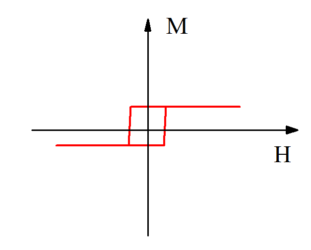
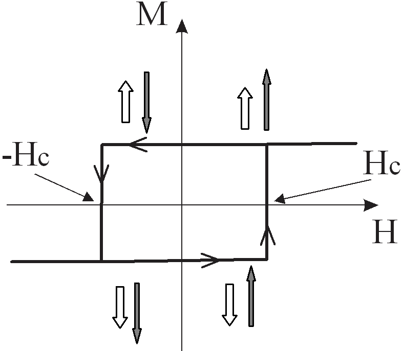

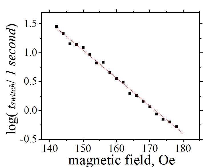
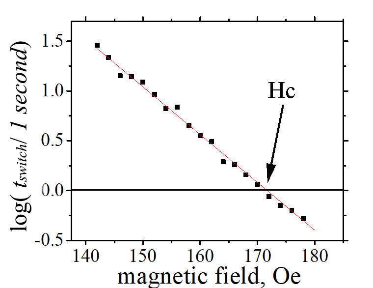
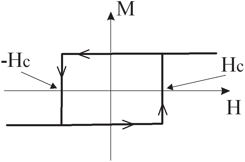

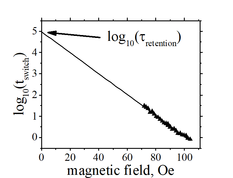
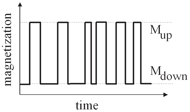

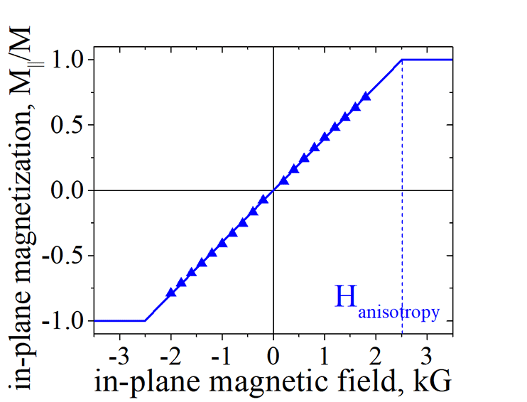
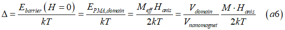
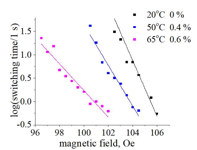
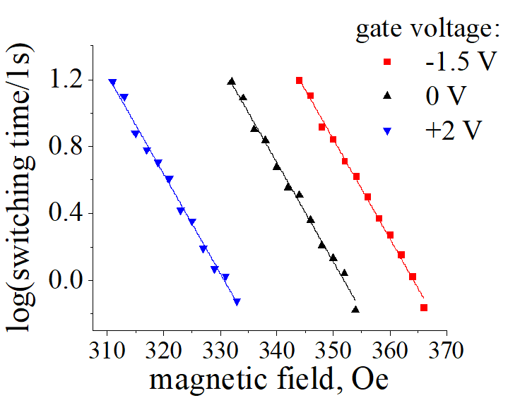
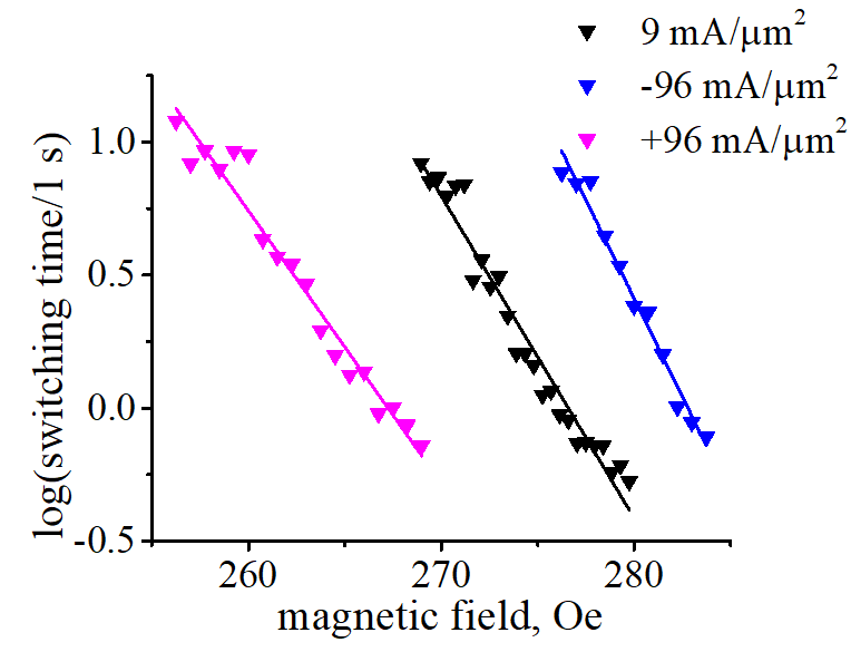
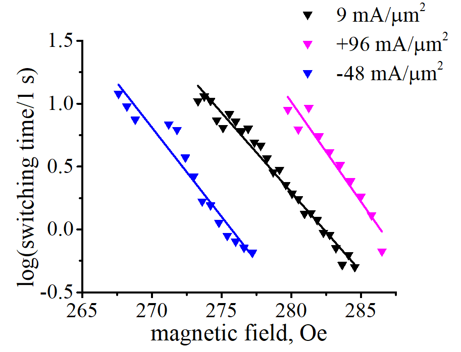

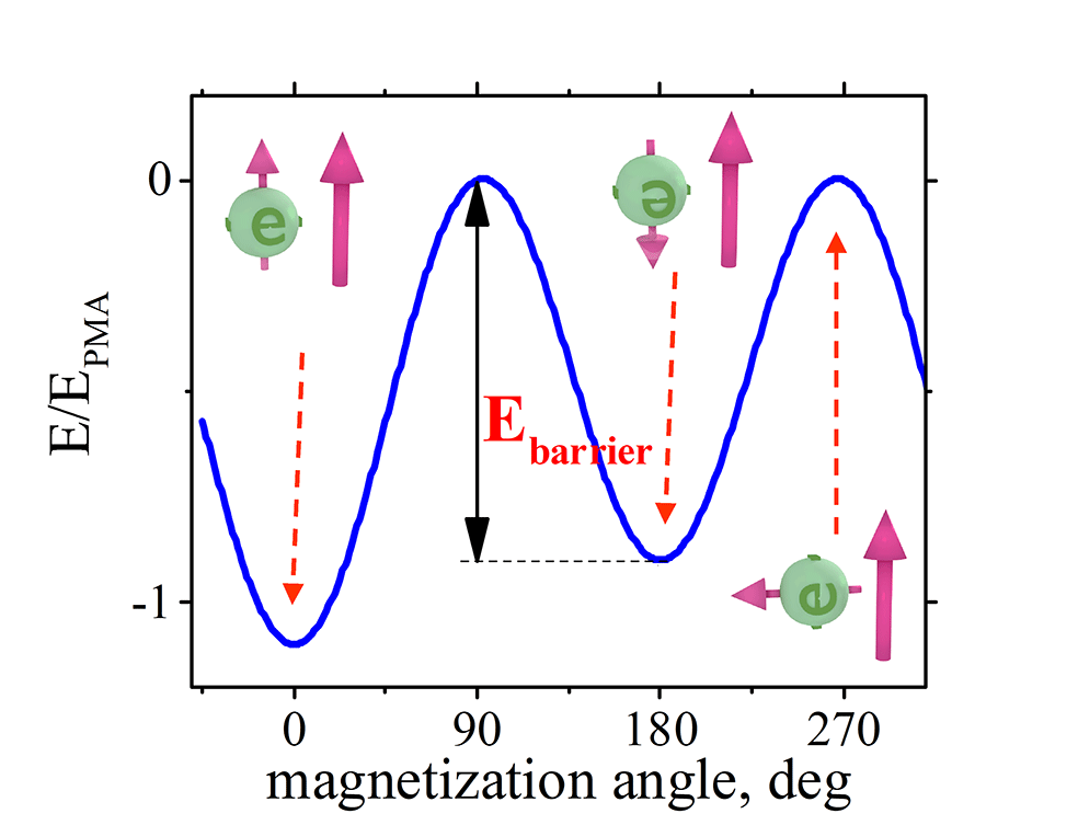
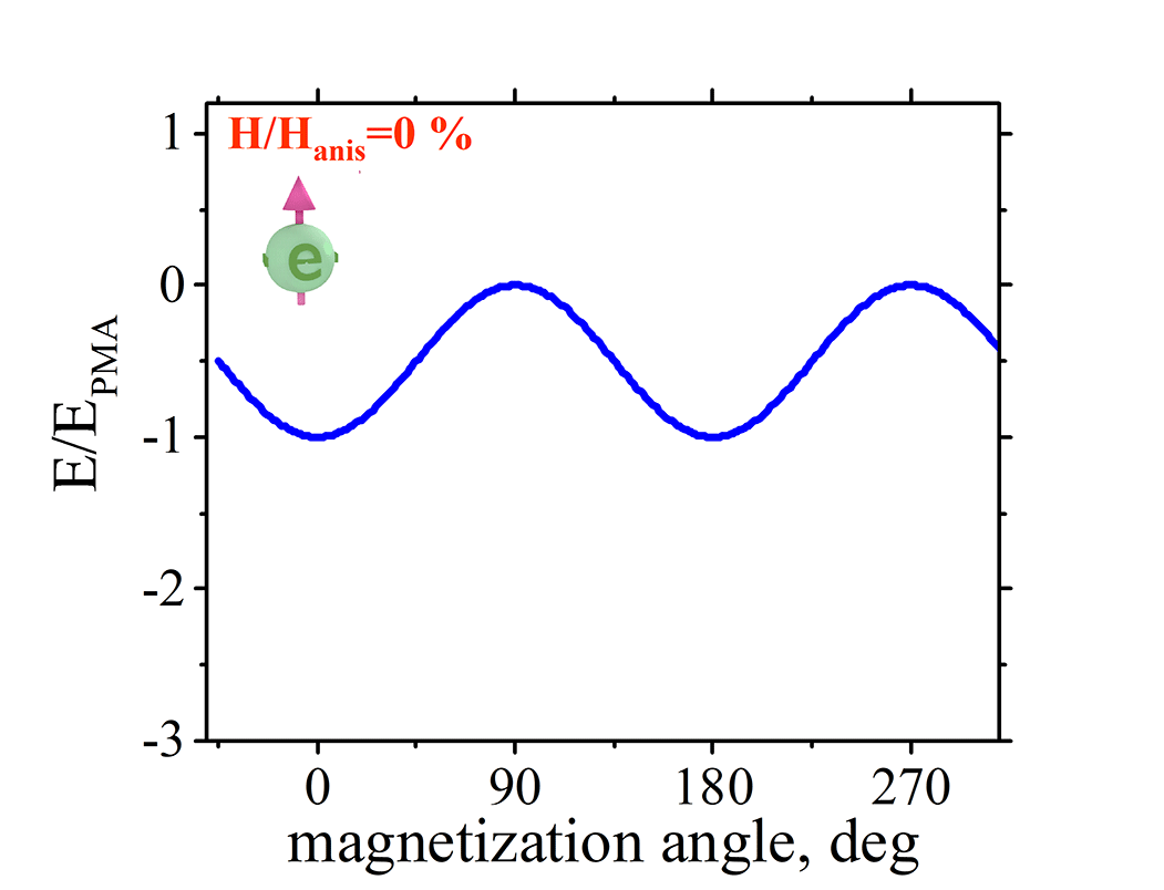
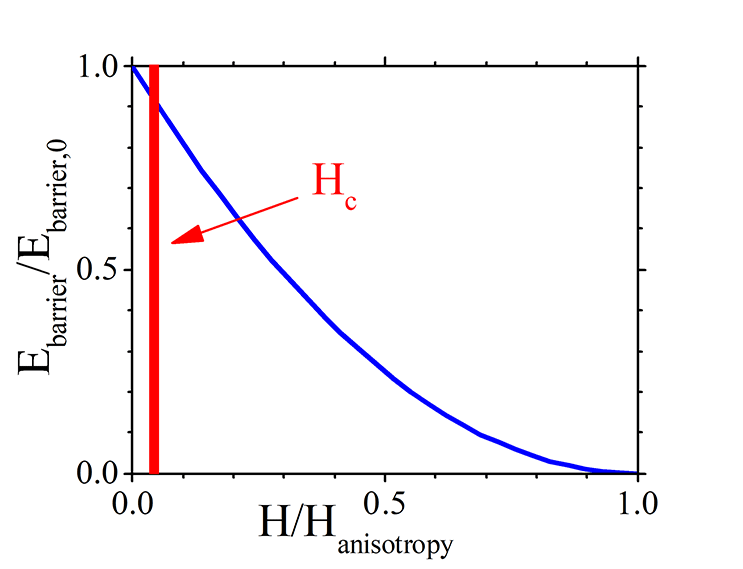
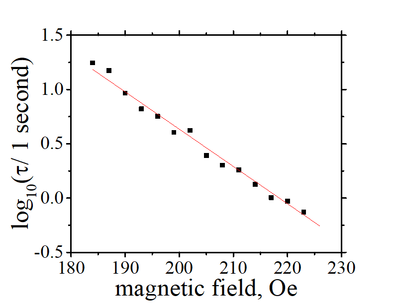
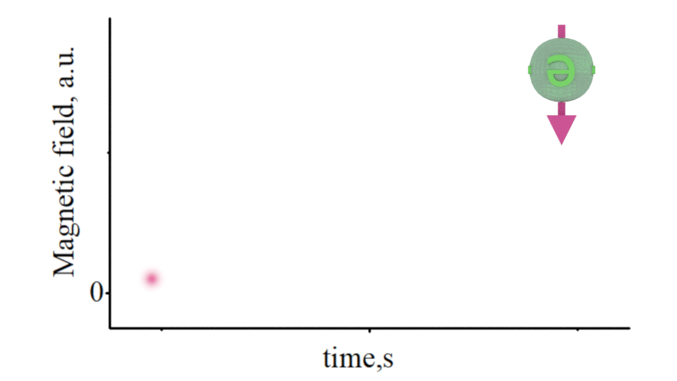
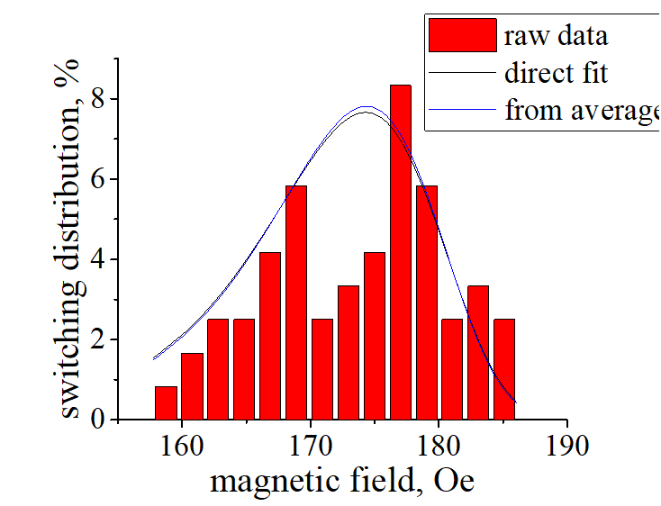
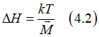
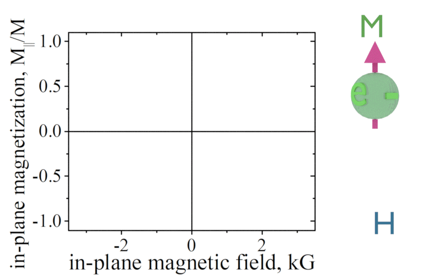
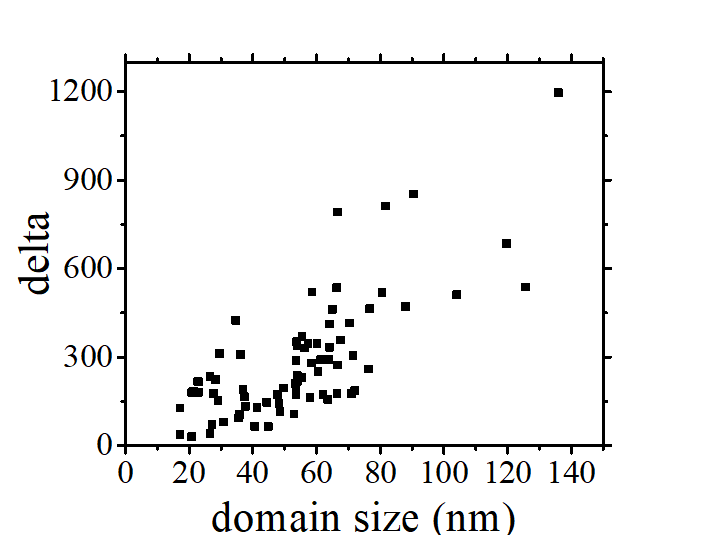
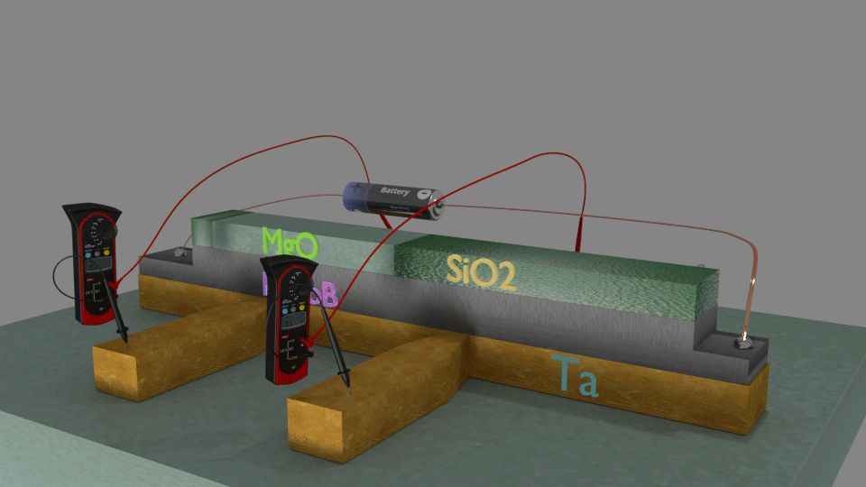
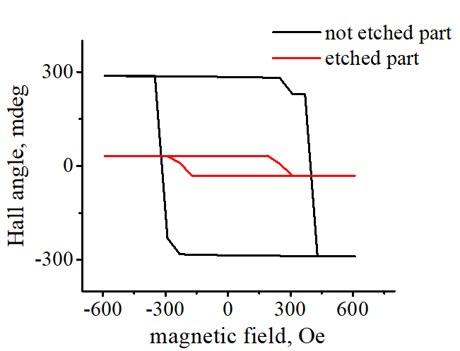
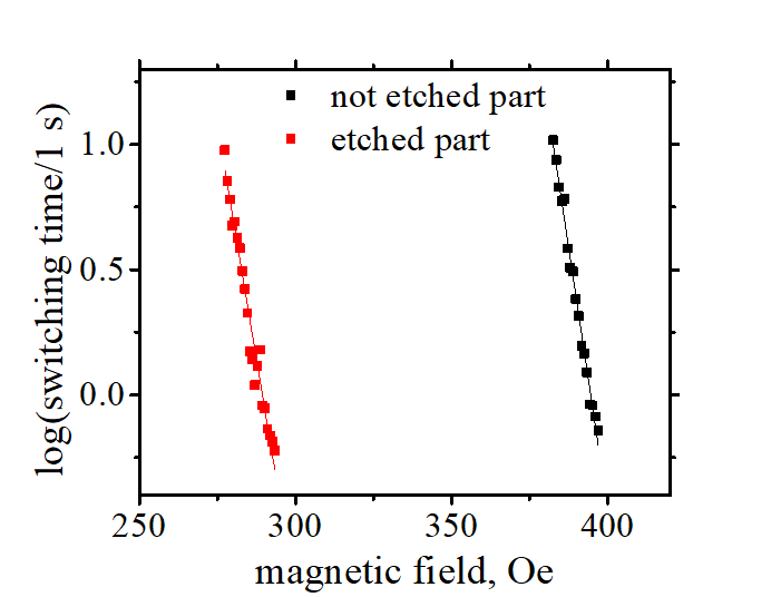
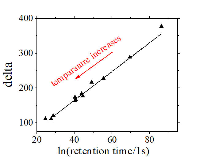
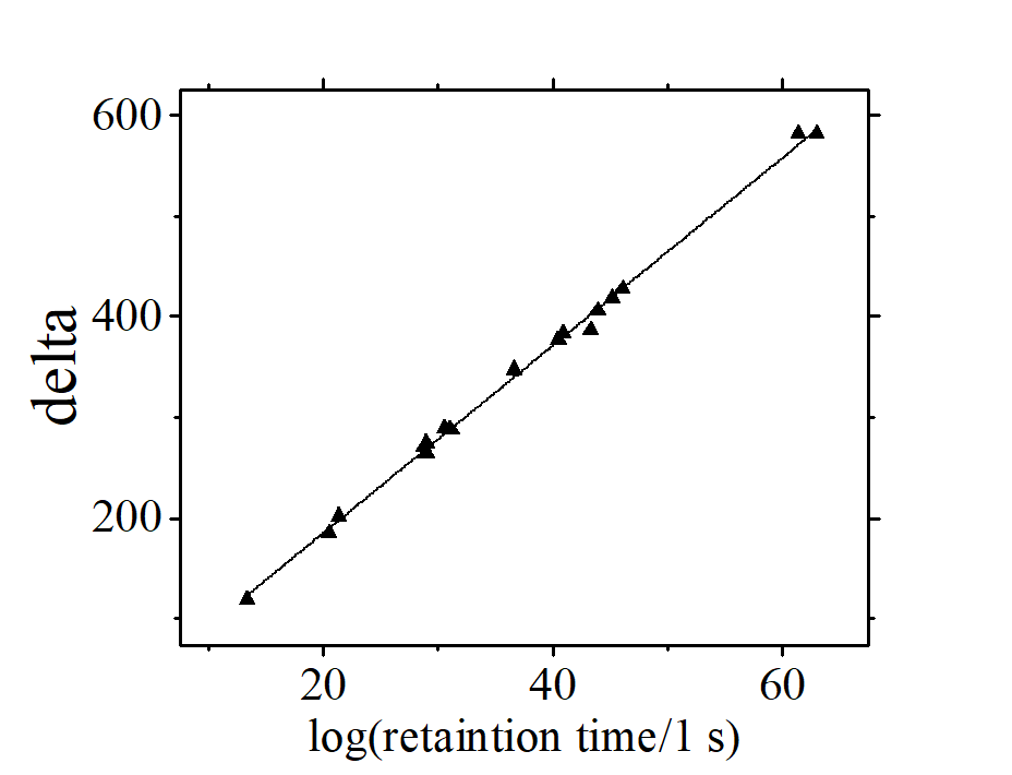
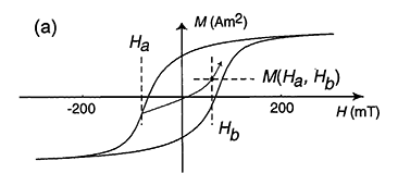
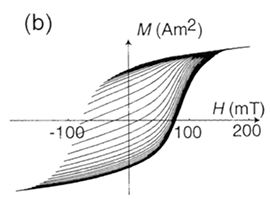
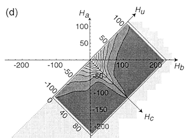
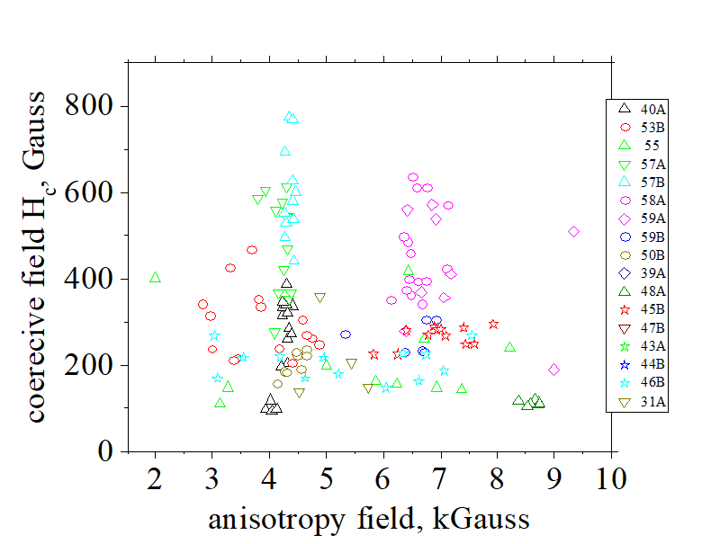
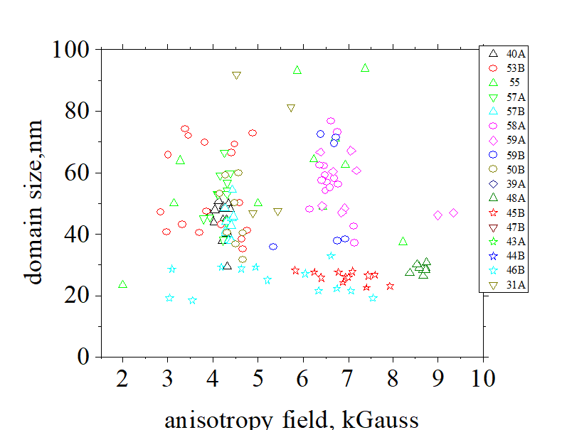
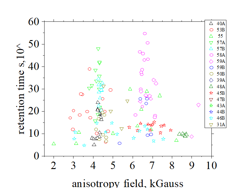
